Class Notes
First Author
1my@email.com
Ernst-August Doelle
1,2Abstract
One or two sentences providing a basic introduction to the field, comprehensible to a scientist in any discipline.
Two to three sentences of more detailed background, comprehensible to scientists in related disciplines.
One sentence clearly stating the general problem being addressed by this particular study.
One sentence summarizing the main result (with the words “here we show” or their equivalent).
Two or three sentences explaining what the main result reveals in direct comparison to what was thought to be the case previously, or how the main result adds to previous knowledge.
One or two sentences to put the results into a more general context.
02/25/19 GGplot2 & dataframes
Table for a data frame: srt dim age subject live 200 dim 17 1 bk 300 bright
Namess<- c("peter","paul","mary",NA)
Ages <- c(1000,1200,100,50) #if you have a 4th variable in only one category then you have to add NA in the others so it equals in length
Sex<- c("M","M","F",NA)

my_df<-data.frame(Names = Namess,
                  Age = Ages,
                  Sex = Sex)
#my_df$ #gives you all the columns

#names is saved as a factor

#my_df$Namess<-as.character(my_df$Namess)
once you get data into a long format table, the graph is easy
library(ggplot2)
# Create dataframe
a <- c(1,2,3,2,3,4,5,4)
b <- c(4,3,4,3,2,1,2,3)
plot_df <- data.frame(a,b)

# basic scatterplot
ggplot(data =plot_df, aes(x=a,y=b))+
  geom_point()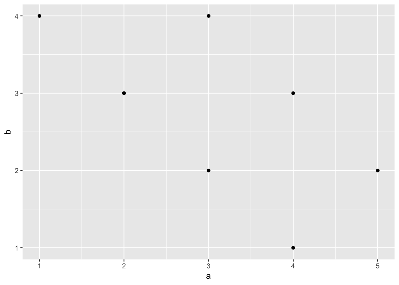
# customize, add regression line
ggplot(data = plot_df, aes(x=a,y=b))+
  geom_point(size=2)+
  geom_smooth(method=lm)+
  coord_cartesian(xlim=c(0,7),ylim=c(0,10))+  #controls the range of the graph (left to right)
  xlab("x-axis label")+
  ylab("y-axis label")+
  ggtitle("I made a scatterplot")+
  theme_classic(base_size=12)+  #changes the background & controls the font size, guaranteeing that it will stay that way.
  theme(plot.title = element_text(hjust = 0.5))
#Create a dataframe
factor_one <- as.factor(c("A","B","C"))
dv_means <- c(20,30,40)
dv_SEs   <- c(4,3.4,4)
plot_df <- data.frame(factor_one,
                      dv_means,
                      dv_SEs)

# basic bar graph

ggplot(plot_df, aes(x=factor_one,y=dv_means))+ #set what will be x axis and what will be the y axis. have a plus to tell it you're adding another layer
  geom_bar(stat="identity") #stat = identity means dont touch the data statistically just plot it as is.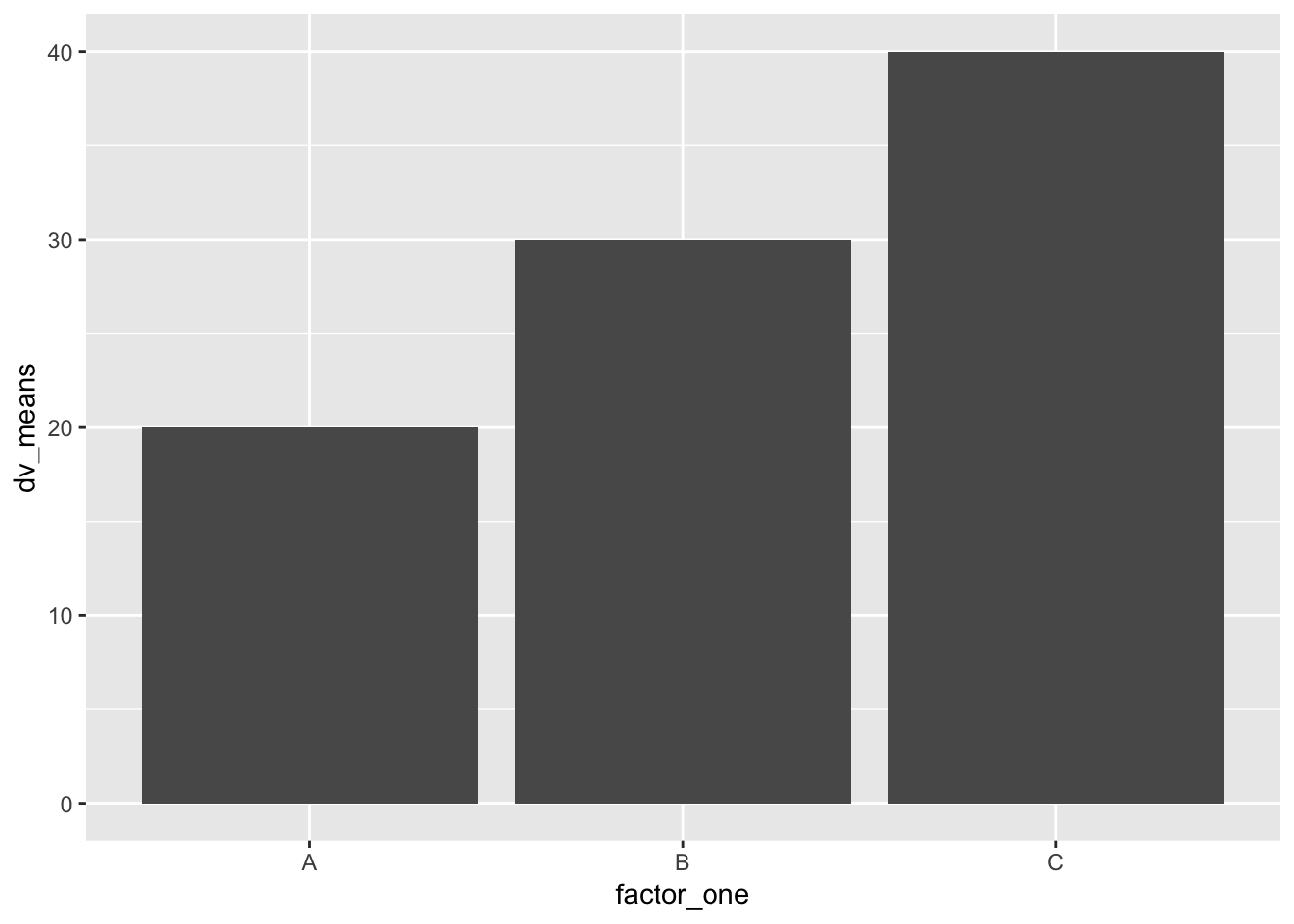
# adding error bars, customizing

ggplot(plot_df, aes(x=factor_one,y=dv_means))+
  geom_bar(stat="identity")+
  geom_errorbar(aes(ymin=dv_means-dv_SEs,
                    ymax=dv_means+dv_SEs),
                width=.2)+
  coord_cartesian(ylim=c(0,100))+
  xlab("x-axis label")+
  ylab("y-axis label")+
  ggtitle("I made a bar graph")+
  theme_classic(base_size=12)+
  theme(plot.title = element_text(hjust = 0.5))
#Create a dataframe
factor_one <- rep(as.factor(c("A","B","C")),2)
factor_two <- rep(as.factor(c("IIA","IIB")),3)
dv_means <- c(20,30,40,20,40,40)
dv_SEs   <- c(4,3.4,4,3,2,4)
plot_df <- data.frame(factor_one,
                      factor_two,
                      dv_means,
                      dv_SEs)

# basic bar graph

ggplot(plot_df, aes(x=factor_one,y=dv_means,
                    group=factor_two,
                    color=factor_two, # color = only for border
                    fill=factor_two))+
  geom_bar(stat="identity", position="dodge",color="black") #dodge makes the bars next to each other, without dodge theyre on top of each other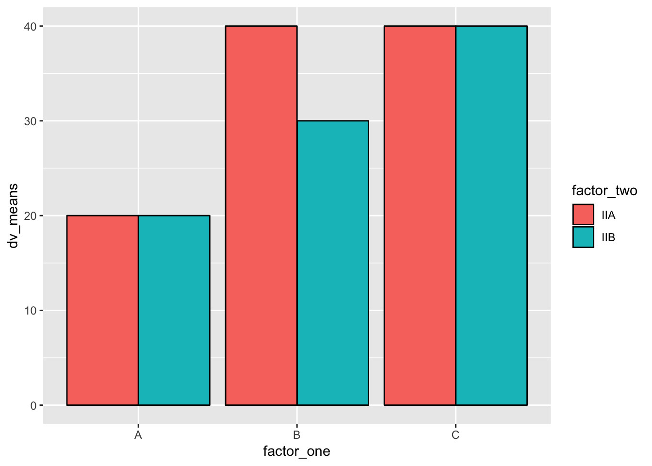
# adding error bars, customizing

ggplot(plot_df, aes(x=factor_one,y=dv_means,
                    group=factor_two,
                    color=factor_two,
                    fill=factor_two))+
  geom_bar(stat="identity", position="dodge")+
  geom_errorbar(aes(ymin=dv_means-dv_SEs,
                    ymax=dv_means+dv_SEs),
                position=position_dodge(width=0.9), #important to make error bars look right
                width=.2,
                color="black")+
  coord_cartesian(ylim=c(0,100))+
  xlab("x-axis label")+
  ylab("y-axis label")+
  ggtitle("Bar graph 2 factors")+
  theme_classic(base_size=12)+
  theme(plot.title = element_text(hjust = 0.5))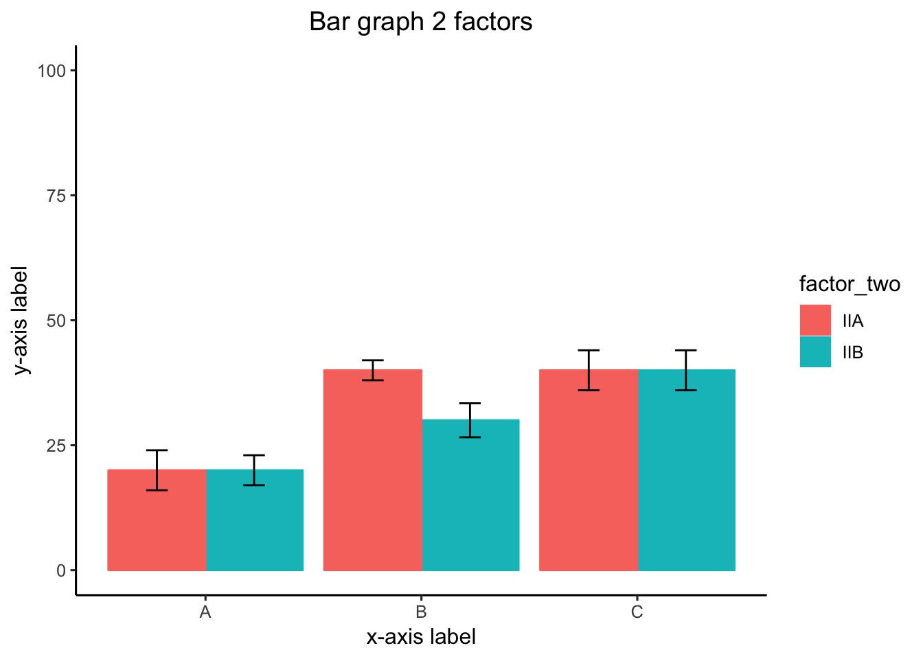
#Create a dataframe
factor_one <- rep(rep(as.factor(c("A","B","C")),2),2)
factor_two <- rep(rep(as.factor(c("IIA","IIB")),3),2)
factor_three <- rep(as.factor(c("IIIA","IIIB")),each=6)
dv_means <- c(20,30,40,20,40,40,
              10,20,50,50,10,10)
dv_SEs   <- c(4,3.4,4,3,2,4,
              1,2,1,2,3,2)
plot_df <- data.frame(factor_one,
                      factor_two,
                      factor_three,
                      dv_means,
                      dv_SEs)

# basic bar graph

ggplot(plot_df, aes(x=factor_one,y=dv_means,
                    group=factor_two,
                    color=factor_two))+
  geom_bar(stat="identity", position="dodge")+
  facet_wrap(~factor_three) # breaks it into 2 graphs
Namez<- rep(c("Dara","Azalea","Barbi","Rowena","Fiona" ),each=2)
MF <- rnorm(10,45,25)
Condition <- rep(c("Social", "Nonsocial"),5)
Aversion <- rep(c("A","N_A"),times=c(4,6))
plot_df<- data.frame(Namez,MF,Condition,Aversion)

ggplot(plot_df, aes(x=Condition, y=MF, group=Namez,linetype=Aversion))+
  geom_line()+
  geom_text(label=Namez)+
  theme_classic()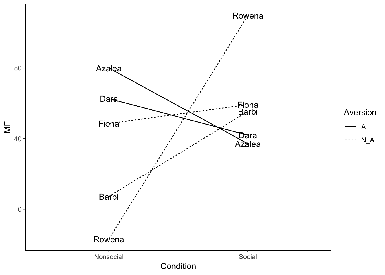
03/04/19 Snow Day
What is Data-wrangling
Data-wrangling is the general process of organizing and transforming data into various formats. For example, loading data into R, pre-processing it to get rid of things you don’t want and keep the things you want, add new things you might want that, arranging the data in different ways to accomplish different kinds of tasks, grouping the data, and summarizing the data, are all common data-wrangling activities. Real-world data often has many imperfections, so data-wrangling is necessary to get the data into a state that is readily analyzable.
We will mainly go over the dplyr package, which has a number of fantastic and relatively easy to use tools for data-wrangling. At the same time, it worth developigng your basic programming skills (using loops and logic), as they are also indispensable for solving unusual data-wrangling problems.
dplyr basics
library(dplyr) #load the package (make sure it is installed first)
df <- starwars # dplyr comes with a data.frame called starwars
Take a look at that data in df, what do you see? It lists various characters from starwars, along with many columns that code for different properties of each character
basic dataframe stuff without dplyr
# addressing specific columns
df$name
df$height
df$mass
# addressing columns and rows without names
df[1,] # row 1
df[,1] # column 1
df[1:4,] # all of the data in rows 1:4
df[,4:5] # all of the data in columns 4:5
df[1:3,6:7] # the data in rows 1 to 3, for column 6 and 7 only
# finding a row(s) with specific info
df[df$name=="Luke Skywalker",]
df[df$height > 180,]
df[df$height < 180 & df$height > 70,]
#replace a particular value
df[1,2] <- 173 #changes the cell in row 1 column 2
# size of dataframe
dim(df) #c(number of rows, number of columns)
# cbind to add a column to a data.frame
df <- cbind(df, random_number=runif(dim(df)[1],0,1))
# rbind to add rows
# this creates a new data frame, binding together the rows 1-2, and 5-6
# note: all of the columns need to be the same
new_df <- rbind(df[1:2,],df[5:6,])
# convert a character vector to a factor
df$species <- as.factor(df$species)
levels(df$species)
levels(df$species)[3] <- "hello" # renames the third level, which get's applied to all listings in the df
A couple questions:
- What are the names of all the characters who are taller than 80, shorter than 140, and are female?
df[df$height > 80 &
     df$height < 170 &
df$gender == "female", ]$name- How many characters have Tatooine for their homeworld?
df[df$homeworld=="Tatooine",]
dim(df[df$homeworld=="Tatooine",])[1] # counts the NAs
tatooine <- df[df$homeworld=="Tatooine",]
tatooine[is.na(tatooine$name)==FALSE,]
dim(tatooine[is.na(tatooine$name)==FALSE,])[1]
dplyr style
We now look at dplyr and pipes. The idea here is that we start with a dataframe, then systematically transform one step at a time. At each step we pass the data in it’s new state to the next step. The passing is called piping the data. There is a special operator for this %>%
quick example
We start with the entire dataframe df. Then we select only the rows where the height is taller than 100. Then we group by homeworld, and compute the mean birth year. What we get is a new data.frame, showing the mean birth years for each homeworld.
This is a common refrain:
Dataframe %>% filter %>% group_by %>% summarise
library(dplyr)

new_df <- df %>%
            filter(height > 100) %>%
            group_by(homeworld) %>%
            summarise(mean_birth_year = mean(birth_year,na.rm=TRUE))
filter
We can filter the data by properties of particular columns
# make a new dataframe that only include rows where the height is greater than 120
new_df <- df %>%
        filter(height > 120)
# multiple filters are seperated by a comma
new_df <- df %>%
        filter(height > 120,
               height < 180,
               birth_year > 20)
# more examples of differen logical operators
new_df <- df %>%
        filter(gender == "male") # == equals identity (same as)
new_df <- df %>%
        filter(gender != "male") # != not equal to
new_df <- df %>%
        filter(eye_color %in% c("blue","yellow") == TRUE) # looks for matches to blue and yellow
# <= less than or equal to
# >= greater than or equal to
new_df <- df %>%
        filter(height >= 120,
               height <= 180)
new_df <- df %>%
        filter(height > 120 & height < 180) # &  AND
new_df <- df %>%
        filter(skin_color == "fair" | skin_color == "gold") # | OR
group_by and summarise
group_by() let’s us grab parts of the data based on the levels in the column
summarise() applies a function to each of the groups that are created
# counts the number of names, for each hair color
new_df <- df %>%
          group_by(hair_color) %>%
          summarise(counts=length(name))
# counts names, for each combination of hair and eye color
new_df <- df %>%
          group_by(hair_color,eye_color) %>%
          summarise(counts=length(name))
focus on summarise
summarise is very powerful. Using summarise we can apply any function we want to each of the groups. This includes intrinsic R functions, and functions of our own design. And, we can add as many as we want. What we get back are new dataframes with columns for each group, and new columns with variables containing the data we want from the analysis
new_df <- df %>%
          group_by(hair_color,eye_color) %>%
          summarise(mean_years = mean(birth_year,na.rm=TRUE),
                    sd_years = sd(birth_year,na.rm=TRUE),
                    counts = length(name))
Mutate
Use mutate to change or add a column
# change numbers in the height column by subtracting 100
library(dplyr)
new_df <- df %>%
            mutate(height=height-100)
# make a new column dividing height by mass
new_df <- df %>%
            mutate(hm_ratio = height/mass)
Select
Use select to select columns of interest and return a dataframe only with those columns
new_df <- df %>%
            select(name,height,mass)
Star wars questions and answers
- use dplyr to find how many movies each character appeared in. Return a table that lists the names, and the number of films
# two ways to do the same thing
new_df <- df %>%
            select(name,films) %>%
            group_by(name) %>%
            mutate(films = length(unlist(films)))
new_df <- df %>%
            select(name,films) %>%
            group_by(name) %>%
summarise(films = length(unlist(films)))- How many characters are in each movie?
- dplyr isn’t always necessary for every question
table(unlist(df$films))##
## A New Hope Attack of the Clones Return of the Jedi
## 18 40 20
## Revenge of the Sith The Empire Strikes Back The Force Awakens
## 34 16 11
## The Phantom Menace
## 34- What is the mean height and mass of characters with blue eyes?
new_df <- df %>%
            filter(eye_color=="blue") %>%
            summarise(mean_height = mean(height,na.rm=TRUE),
                      mean_mass = mean(mass,na.rm=TRUE))
Data input
Before we wrangle with data, we need to get it into R. There are many ways to do that.
All of the following examples assume you have a data folder in your workspace that contains all the data files we will be using. Download this .zip file https://github.com/CrumpLab/statisticsLab/raw/master/RstudioCloud.zip. Unzip the file. Then copy the data folder into your R markdown project folder.
WARNING: loading files requires you to tell R exactly where the file is on your computer. This can involve specifying the entire file path (the drive, all of the folder, and then the filename). These examples avoid this complete filename nonsense by putting the files in a data folder in your R project folder. Then, we just need to specify the folder and the filename. In this case, the folder will always be data. In general, R by default attempts to load files from the current working directory, which is automatically set to your project folder when you are working in an R-studio project.
# loading a csv file using read.csv
hsq <- read.csv("RstudioCloud/data/hsq.csv")
# alternative using fread
library(data.table)
hsq <- fread("RstudioCloud/data/hsq.csv") # creates a data.table, similar to a data.frame
# loading an SPSS sav file
library(foreign)
spss <- read.spss("RstudioCloud/data/02_NYC_Salary_City_2016.sav",
                  to.data.frame=TRUE)
Other helpful libraries for reading in files
- libary
readxllet’s you read in excel files - library
googlesheetslet’s you read in google spreadsheets - function
scanis a powerful and all purpose text input function, often helpful in very messy situations where you want to read in line-by-line loadfor R data files- there are several
read.functions for specific situations. - library
jsonlitefor json data structures - and many more, this is really something that you will learn more about on a case-by-case basis as you have to deal with particular data formats.
03/11/19 Going over data wrangling
#strs(stimulus[1], split="")fig.path = “myfigs/”, dev = c(“pdf”, “png”)
^^ use in 1st chunk to save graphs
03/18/19 Statistics
Discussing midterm assignment Part 1 (due April 1) 1. make a new github repository. put work into it. 2. find a psych paper with open data. - osf.io = open science framework - psychological science (look for blue badge) journals.sagepub.com - crumplab/statistics lab 3. load into r 4. re-analyse the data to see if you can reproduce the results from the original paper 5. write it up in reproducible report (.rmd file)
Part 2 (due April 1) 1. Convert your reproducible report into an APA style research report using papaja package.
Part 3 (due April 8) 1. Add a section following the results where you conduct and report a simulation based power analysis
The most important thing about choosing statistics, is being able to justify the statistics that you choose.
There are many tools in the toolbox. There are many recommendations about what to do or not to do. It is a good idea to understand the statistics that you use, so that you can justify why you are using them for your analysis.
t-tests
one sample t-test
Set mu to test against a population value
x <- c(1,4,3,2,3,4,3,2,3,2,3,4)
#non-directional
t.test(x, mu = 2)
##
## One Sample t-test
##
## data: x
## t = 3.0794, df = 11, p-value = 0.01048
## alternative hypothesis: true mean is not equal to 2
## 95 percent confidence interval:
## 2.237714 3.428952
## sample estimates:
## mean of x
## 2.833333t.test(x, mu = 2, alternative = "two.sided") # the default##
## One Sample t-test
##
## data: x
## t = 3.0794, df = 11, p-value = 0.01048
## alternative hypothesis: true mean is not equal to 2
## 95 percent confidence interval:
## 2.237714 3.428952
## sample estimates:
## mean of x
## 2.833333# directional
t.test(x, mu = 2, alternative = "greater")##
## One Sample t-test
##
## data: x
## t = 3.0794, df = 11, p-value = 0.005241
## alternative hypothesis: true mean is greater than 2
## 95 percent confidence interval:
## 2.34734 Inf
## sample estimates:
## mean of x
## 2.833333t.test(x, mu = 2, alternative = "less")##
## One Sample t-test
##
## data: x
## t = 3.0794, df = 11, p-value = 0.9948
## alternative hypothesis: true mean is less than 2
## 95 percent confidence interval:
## -Inf 3.319326
## sample estimates:
## mean of x
## 2.833333t = mean/SEM SEM tells you how things vary
paired-sample t-test
Set paired=TRUE
x <- c(1,4,3,2,3,4,3,2,3,2,3,4)
y <- c(3,2,5,4,3,2,3,2,1,2,2,3)
#non-directional
t.test(x, y, paired=TRUE)
##
## Paired t-test
##
## data: x and y
## t = 0.37796, df = 11, p-value = 0.7126
## alternative hypothesis: true difference in means is not equal to 0
## 95 percent confidence interval:
## -0.8038766 1.1372099
## sample estimates:
## mean of the differences
## 0.1666667t.test(x, y, paired=TRUE, alternative = "two.sided") # the default##
## Paired t-test
##
## data: x and y
## t = 0.37796, df = 11, p-value = 0.7126
## alternative hypothesis: true difference in means is not equal to 0
## 95 percent confidence interval:
## -0.8038766 1.1372099
## sample estimates:
## mean of the differences
## 0.1666667# directional
t.test(x, y, paired=TRUE, alternative = "greater")##
## Paired t-test
##
## data: x and y
## t = 0.37796, df = 11, p-value = 0.3563
## alternative hypothesis: true difference in means is greater than 0
## 95 percent confidence interval:
## -0.6252441 Inf
## sample estimates:
## mean of the differences
## 0.1666667t.test(x, y, paired=TRUE, alternative = "less")##
## Paired t-test
##
## data: x and y
## t = 0.37796, df = 11, p-value = 0.6437
## alternative hypothesis: true difference in means is less than 0
## 95 percent confidence interval:
## -Inf 0.9585774
## sample estimates:
## mean of the differences
## 0.1666667Independent sample t-test
Note: Default is Welch test, set var.equal=TRUE for t-test
x <- c(1,4,3,2,3,4,3,2,3,2,3,4)
y <- c(3,2,5,4,3,2,3,2,1,2,2,3)
#non-directional
t.test(x, y, var.equal=TRUE)
##
## Two Sample t-test
##
## data: x and y
## t = 0.40519, df = 22, p-value = 0.6893
## alternative hypothesis: true difference in means is not equal to 0
## 95 percent confidence interval:
## -0.6863784 1.0197117
## sample estimates:
## mean of x mean of y
## 2.833333 2.666667t.test(x, y, var.equal=TRUE, alternative = "two.sided") # the default##
## Two Sample t-test
##
## data: x and y
## t = 0.40519, df = 22, p-value = 0.6893
## alternative hypothesis: true difference in means is not equal to 0
## 95 percent confidence interval:
## -0.6863784 1.0197117
## sample estimates:
## mean of x mean of y
## 2.833333 2.666667# directional
t.test(x, y, var.equal=TRUE, alternative = "greater")##
## Two Sample t-test
##
## data: x and y
## t = 0.40519, df = 22, p-value = 0.3446
## alternative hypothesis: true difference in means is greater than 0
## 95 percent confidence interval:
## -0.5396454 Inf
## sample estimates:
## mean of x mean of y
## 2.833333 2.666667t.test(x, y, var.equal=TRUE, alternative = "less")##
## Two Sample t-test
##
## data: x and y
## t = 0.40519, df = 22, p-value = 0.6554
## alternative hypothesis: true difference in means is less than 0
## 95 percent confidence interval:
## -Inf 0.8729787
## sample estimates:
## mean of x mean of y
## 2.833333 2.666667printing
library(broom)
t_results <- t.test(x, y, var.equal=TRUE)
knitr::kable(tidy(t_results))| estimate1 | estimate2 | statistic | p.value | parameter | conf.low | conf.high | method | alternative |
|---|---|---|---|---|---|---|---|---|
| 2.833333 | 2.666667 | 0.4051902 | 0.6892509 | 22 | -0.6863784 | 1.019712 | Two Sample t-test | two.sided |
writing
The contents of R variables can be written into R Markdown documents.
t(22) =0.41, p = 0.689
# write your own function
report_t <- function(x){
  return(paste(c("t(",round(x$parameter, digits=2),") ",
        "= ",round(x$statistic, digits=2),", ",
        "p = ",round(x$p.value, digits=3)), collapse=""))
}
report_t(t_results)
## [1] "t(22) = 0.41, p = 0.689"t_results##
## Two Sample t-test
##
## data: x and y
## t = 0.40519, df = 22, p-value = 0.6893
## alternative hypothesis: true difference in means is not equal to 0
## 95 percent confidence interval:
## -0.6863784 1.0197117
## sample estimates:
## mean of x mean of y
## 2.833333 2.666667The results of my t-test were t(22) = 0.41, p = 0.689.
ANOVA
F = T^2
Effect/Error
SS_Effect/DF1 –> M^2 Eff / SS_Error/DF2 –> M^2 Error
Requires data to be in long-format.
# example creation of 2x2 data
Subjects <- rep(1:10,each=4)
Factor1 <- rep(rep(c("A","B"), each = 2), 10)
Factor2 <- rep(rep(c("1","2"), 2), 10)
DV <- rnorm(40,0,1)
all_data <- data.frame(Subjects = as.factor(Subjects),
                       DV,
                       Factor1,
                       Factor2)
between-subjects 1 factor
# run anova
aov_out <- aov(DV~Factor1, all_data)
# summary
sum_out <- summary(aov_out)
# kable xtable printing
library(xtable)
knitr::kable(xtable(summary(aov_out)))| Df | Sum Sq | Mean Sq | F value | Pr(>F) | |
|---|---|---|---|---|---|
| Factor1 | 1 | 0.9712296 | 0.9712296 | 1.071932 | 0.3070536 |
| Residuals | 38 | 34.4301122 | 0.9060556 | NA | NA |
# print means
print(model.tables(aov_out,"means"), format="markdown")
## Tables of means
## Grand mean
##
## -0.1673187
##
## Factor1
## Factor1
## A B
## -0.3231 -0.0115sum_out[[1]]$`F value`[1]## [1] 1.071932#kable function good for making dataframes into pretty tablebetween-subjects 2 factor
# run anova
aov_out <- aov(DV~Factor1*Factor2, all_data)
# summary
summary(aov_out)
## Df Sum Sq Mean Sq F value Pr(>F)
## Factor1 1 0.97 0.9712 1.093 0.303
## Factor2 1 1.39 1.3881 1.562 0.219
## Factor1:Factor2 1 1.05 1.0498 1.181 0.284
## Residuals 36 31.99 0.8887# kable xtable printing
library(xtable)
knitr::kable(xtable(summary(aov_out)))| Df | Sum Sq | Mean Sq | F value | Pr(>F) | |
|---|---|---|---|---|---|
| Factor1 | 1 | 0.9712296 | 0.9712296 | 1.092898 | 0.3027991 |
| Factor2 | 1 | 1.3880989 | 1.3880989 | 1.561989 | 0.2194384 |
| Factor1:Factor2 | 1 | 1.0497591 | 1.0497591 | 1.181265 | 0.2843224 |
| Residuals | 36 | 31.9922542 | 0.8886737 | NA | NA |
# print means
print(model.tables(aov_out,"means"), format="markdown")
## Tables of means
## Grand mean
##
## -0.1673187
##
## Factor1
## Factor1
## A B
## -0.3231 -0.0115
##
## Factor2
## Factor2
## 1 2
## 0.0190 -0.3536
##
## Factor1:Factor2
## Factor2
## Factor1 1 2
## A 0.0251 -0.6714
## B 0.0128 -0.0358repeated-measures 1 factor
# run anova
aov_out <- aov(DV~Factor1 + Error(Subjects/Factor1), all_data)
# summary
summary(aov_out)
##
## Error: Subjects
## Df Sum Sq Mean Sq F value Pr(>F)
## Residuals 9 4.337 0.4819
##
## Error: Subjects:Factor1
## Df Sum Sq Mean Sq F value Pr(>F)
## Factor1 1 0.971 0.9712 0.496 0.499
## Residuals 9 17.620 1.9578
##
## Error: Within
## Df Sum Sq Mean Sq F value Pr(>F)
## Residuals 20 12.47 0.6237# kable xtable printing
library(xtable)
knitr::kable(xtable(summary(aov_out)))| Df | Sum Sq | Mean Sq | F value | Pr(>F) | |
|---|---|---|---|---|---|
| Residuals | 9 | 4.3369481 | 0.4818831 | NA | NA |
| Factor1 | 1 | 0.9712296 | 0.9712296 | 0.4960939 | 0.4990397 |
| Residuals1 | 9 | 17.6197832 | 1.9577537 | NA | NA |
| Residuals2 | 20 | 12.4733808 | 0.6236690 | NA | NA |
# print means
print(model.tables(aov_out,"means"), format="markdown")
## Tables of means
## Grand mean
##
## -0.1673187
##
## Factor1
## Factor1
## A B
## -0.3231 -0.0115repeated-measures 2 factor
# run anova
aov_out <- aov(DV~Factor1*Factor2 + Error(Subjects/(Factor1*Factor2)), all_data)
# summary
summary(aov_out)
##
## Error: Subjects
## Df Sum Sq Mean Sq F value Pr(>F)
## Residuals 9 4.337 0.4819
##
## Error: Subjects:Factor1
## Df Sum Sq Mean Sq F value Pr(>F)
## Factor1 1 0.971 0.9712 0.496 0.499
## Residuals 9 17.620 1.9578
##
## Error: Subjects:Factor2
## Df Sum Sq Mean Sq F value Pr(>F)
## Factor2 1 1.388 1.3881 1.726 0.221
## Residuals 9 7.239 0.8043
##
## Error: Subjects:Factor1:Factor2
## Df Sum Sq Mean Sq F value Pr(>F)
## Factor1:Factor2 1 1.050 1.0498 3.378 0.0992 .
## Residuals 9 2.797 0.3108
## ---
## Signif. codes: 0 '***' 0.001 '**' 0.01 '*' 0.05 '.' 0.1 ' ' 1# kable xtable printing
library(xtable)
knitr::kable(xtable(summary(aov_out)))| Df | Sum Sq | Mean Sq | F value | Pr(>F) | |
|---|---|---|---|---|---|
| Residuals | 9 | 4.3369481 | 0.4818831 | NA | NA |
| Factor1 | 1 | 0.9712296 | 0.9712296 | 0.4960939 | 0.4990397 |
| Residuals1 | 9 | 17.6197832 | 1.9577537 | NA | NA |
| Factor2 | 1 | 1.3880989 | 1.3880989 | 1.7258326 | 0.2214434 |
| Residuals2 | 9 | 7.2387614 | 0.8043068 | NA | NA |
| Factor1:Factor2 | 1 | 1.0497591 | 1.0497591 | 3.3781328 | 0.0992313 |
| Residuals | 9 | 2.7967614 | 0.3107513 | NA | NA |
# print means
print(model.tables(aov_out,"means"), format="markdown")
## Tables of means
## Grand mean
##
## -0.1673187
##
## Factor1
## Factor1
## A B
## -0.3231 -0.0115
##
## Factor2
## Factor2
## 1 2
## 0.0190 -0.3536
##
## Factor1:Factor2
## Factor2
## Factor1 1 2
## A 0.0251 -0.6714
## B 0.0128 -0.0358papaja
#library(papaja)
#apa_stuff <- apa_print.aov(aov_out)
#The main effect for factor 1 was, `r apa_stuff$statistic$Factor1`. The main effect for factor 2 was, `r apa_stuff$statistic$Factor2`. The interaction was, `r apa_stuff$statistic$Factor1_Factor2`Linear Regression
lm(DV~Factor1, all_data)##
## Call:
## lm(formula = DV ~ Factor1, data = all_data)
##
## Coefficients:
## (Intercept) Factor1B
## -0.3231 0.3116summary(lm(DV~Factor1, all_data))##
## Call:
## lm(formula = DV ~ Factor1, data = all_data)
##
## Residuals:
## Min 1Q Median 3Q Max
## -1.61382 -0.56094 -0.09081 0.73849 2.01264
##
## Coefficients:
## Estimate Std. Error t value Pr(>|t|)
## (Intercept) -0.3231 0.2128 -1.518 0.137
## Factor1B 0.3116 0.3010 1.035 0.307
##
## Residual standard error: 0.9519 on 38 degrees of freedom
## Multiple R-squared: 0.02743, Adjusted R-squared: 0.001841
## F-statistic: 1.072 on 1 and 38 DF, p-value: 0.3071lm(DV~Factor1+Factor2, all_data)##
## Call:
## lm(formula = DV ~ Factor1 + Factor2, data = all_data)
##
## Coefficients:
## (Intercept) Factor1B Factor22
## -0.1369 0.3116 -0.3726summary(lm(DV~Factor1+Factor2, all_data))##
## Call:
## lm(formula = DV ~ Factor1 + Factor2, data = all_data)
##
## Residuals:
## Min 1Q Median 3Q Max
## -1.80011 -0.67105 -0.06665 0.60334 1.82635
##
## Coefficients:
## Estimate Std. Error t value Pr(>|t|)
## (Intercept) -0.1369 0.2588 -0.529 0.600
## Factor1B 0.3116 0.2988 1.043 0.304
## Factor22 -0.3726 0.2988 -1.247 0.220
##
## Residual standard error: 0.945 on 37 degrees of freedom
## Multiple R-squared: 0.06665, Adjusted R-squared: 0.01619
## F-statistic: 1.321 on 2 and 37 DF, p-value: 0.2792lm(DV~Factor1*Factor2, all_data)##
## Call:
## lm(formula = DV ~ Factor1 * Factor2, data = all_data)
##
## Coefficients:
## (Intercept) Factor1B Factor22
## 0.02514 -0.01235 -0.69657
## Factor1B:Factor22
## 0.64800summary(lm(DV~Factor1*Factor2, all_data))##
## Call:
## lm(formula = DV ~ Factor1 * Factor2, data = all_data)
##
## Residuals:
## Min 1Q Median 3Q Max
## -1.63811 -0.60893 -0.09186 0.67585 1.66435
##
## Coefficients:
## Estimate Std. Error t value Pr(>|t|)
## (Intercept) 0.02514 0.29811 0.084 0.933
## Factor1B -0.01235 0.42159 -0.029 0.977
## Factor22 -0.69657 0.42159 -1.652 0.107
## Factor1B:Factor22 0.64800 0.59621 1.087 0.284
##
## Residual standard error: 0.9427 on 36 degrees of freedom
## Multiple R-squared: 0.0963, Adjusted R-squared: 0.02099
## F-statistic: 1.279 on 3 and 36 DF, p-value: 0.2964Randomization Test
A <- c(1,2,3,4,5,6,7,8,9,10)
B <- c(2,4,6,8,10,12,14,16,18,20)
all <- c(A,B)
mean_difference <- c()
for(i in 1:10000){
  shuffle <- sample(all)
  newA <- shuffle[1:10]
  newB <- shuffle[11:20]
  mean_difference[i] <- mean(newB)-mean(newA)
}
observed <- mean(B)-mean(A)
length(mean_difference[mean_difference >= observed])/10000
## [1] 0.0121library(EnvStats)
twoSamplePermutationTestLocation(x=B, y=A, fcn = "mean",
alternative = "greater",
mu1.minus.mu2 = 0,
paired = FALSE,
exact = FALSE,
n.permutations = 10000,
seed = NULL,
tol = sqrt(.Machine$double.eps))##
## Results of Hypothesis Test
## --------------------------
##
## Null Hypothesis: mu.x-mu.y = 0
##
## Alternative Hypothesis: True mu.x-mu.y is greater than 0
##
## Test Name: Two-Sample Permutation Test
## Based on Differences in Means
## (Based on Sampling
## Permutation Distribution
## 10000 Times)
##
## Estimated Parameter(s): mean of x = 11.0
## mean of y = 5.5
##
## Data: x = B
## y = A
##
## Sample Sizes: nx = 10
## ny = 10
##
## Test Statistic: mean.x - mean.y = 5.5
##
## P-value: 0.0111Correlation
x <- rnorm(10,0,1)
y <- rnorm(10,0,1)
cor(x,y)
## [1] -0.5337205ranks1 <- sample(1:10)
ranks2 <- sample(1:10)
cor(ranks1,ranks2, method = "spearman")## [1] -0.1393939Chi-square
M <- as.table(rbind(c(762, 327, 468), c(484, 239, 477)))
dimnames(M) <- list(gender = c("F", "M"),
                    party = c("Democrat","Independent", "Republican"))
(Xsq <- chisq.test(M))
##
## Pearson's Chi-squared test
##
## data: M
## X-squared = 30.07, df = 2, p-value = 2.954e-07binomial test
number_of_successes <- 100
trials <- 150
binom.test(x=number_of_successes, n=trials, p = 0.5,
           alternative = "two.sided",
           conf.level = 0.95)
##
## Exact binomial test
##
## data: number_of_successes and trials
## number of successes = 100, number of trials = 150, p-value =
## 5.448e-05
## alternative hypothesis: true probability of success is not equal to 0.5
## 95 percent confidence interval:
## 0.5851570 0.7414436
## sample estimates:
## probability of success
## 0.6666667Post-hoc tests
Many kinds of post-hoc tests can be done in R using base R functions, or functions from other packages.
At the same time, it is common for post-hoc comparison functions to be limited and specific in their functionality. So, if you can’t find an existing function to complete the analysis you want, you may have to modify, extend, or write your own function to do the job.
pairwise t-tests
Performs all possible t-tests between the levels of a grouping factor. Can implement different corrections for multiple comparisons.
df <- airquality #loads the airquality data from base R
df$Month <- as.factor(df$Month)
# default uses holm correction
pairwise.t.test(df$Ozone,df$Month)
##
## Pairwise comparisons using t tests with pooled SD
##
## data: df$Ozone and df$Month
##
## 5 6 7 8
## 6 1.00000 - - -
## 7 0.00026 0.05113 - -
## 8 0.00019 0.04987 1.00000 -
## 9 1.00000 1.00000 0.00488 0.00388
##
## P value adjustment method: holm# use bonferroni correction
pairwise.t.test(df$Ozone,df$Month, p.adj="bonf")##
## Pairwise comparisons using t tests with pooled SD
##
## data: df$Ozone and df$Month
##
## 5 6 7 8
## 6 1.00000 - - -
## 7 0.00029 0.10225 - -
## 8 0.00019 0.08312 1.00000 -
## 9 1.00000 1.00000 0.00697 0.00485
##
## P value adjustment method: bonferronitukey HSD test
notes: the warpbreaks data.frame should be available in base R, you do not need to load it to be able to use it.
Doesn’t work with repeated measures ANOVAs.
summary(fm1 <- aov(breaks ~ wool + tension, data = warpbreaks))## Df Sum Sq Mean Sq F value Pr(>F)
## wool 1 451 450.7 3.339 0.07361 .
## tension 2 2034 1017.1 7.537 0.00138 **
## Residuals 50 6748 135.0
## ---
## Signif. codes: 0 '***' 0.001 '**' 0.01 '*' 0.05 '.' 0.1 ' ' 1TukeyHSD(fm1, "tension", ordered = TRUE)## Tukey multiple comparisons of means
## 95% family-wise confidence level
## factor levels have been ordered
##
## Fit: aov(formula = breaks ~ wool + tension, data = warpbreaks)
##
## $tension
## diff lwr upr p adj
## M-H 4.722222 -4.6311985 14.07564 0.4474210
## L-H 14.722222 5.3688015 24.07564 0.0011218
## L-M 10.000000 0.6465793 19.35342 0.0336262Fishers LSD
Explanation of Fisher’s least significant difference test. https://www.utd.edu/~herve/abdi-LSD2010-pretty.pdf
library(agricolae)
data(sweetpotato)
model <- aov(yield~virus, data=sweetpotato)
out   <- LSD.test(model,"virus", p.adj="bonferroni")
Linear Contrasts
# Create data for a one-way BW subjects, 4 groups
A <- rnorm(n=10, mean=100, sd=25)
B <- rnorm(n=10, mean=120, sd=25)
C <- rnorm(n=10, mean=140, sd=25)
D <- rnorm(n=10, mean=80, sd=25)
DV <- c(A,B,C,D)
Conditions <- as.factor(rep(c("A","B","C","D"), each=10))
df <- data.frame(DV,Conditions)
# one-way ANOVA
aov_out <- aov(DV~Conditions, df)
summary(aov_out)
## Df Sum Sq Mean Sq F value Pr(>F)
## Conditions 3 22572 7524 13.83 3.72e-06 ***
## Residuals 36 19589 544
## ---
## Signif. codes: 0 '***' 0.001 '**' 0.01 '*' 0.05 '.' 0.1 ' ' 1# look at the order of levels
levels(df$Conditions)## [1] "A" "B" "C" "D"# set up linear contrasts
c1 <- c(.5, -.5, -.5, .5) # AD vs. BC
c2 <- c(0, 0, 1, -1) # C vs. D
c3 <- c(0, -1, 1, 0) # B vs. C
# create a contrast matrix
mat <- cbind(c1,c2,c3)
# assign the contrasts to the group
contrasts(df$Conditions) <- mat
# run the ANOVA
aov_out <- aov(DV~Conditions, df)
# print the contrasts, add names for the contrasts
summary.aov(aov_out, split=list(Conditions=list("AD vs. BC"=1, "C vs. D" = 2, "B vs. C"=3))) ## Df Sum Sq Mean Sq F value Pr(>F)
## Conditions 3 22572 7524 13.827 3.72e-06 ***
## Conditions: AD vs. BC 1 18552 18552 34.093 1.14e-06 ***
## Conditions: C vs. D 1 4007 4007 7.365 0.0101 *
## Conditions: B vs. C 1 12 12 0.023 0.8812
## Residuals 36 19589 544
## ---
## Signif. codes: 0 '***' 0.001 '**' 0.01 '*' 0.05 '.' 0.1 ' ' 1a <- replicate(10000,t.test(rnorm(10,0,1))$p.value)
hist(a)
length(a[a<.05])## [1] 546Fact1 <- rep(c("A", "B", "C"), each=5)
DV <- rnorm(n=15, mean=0, sd=1)
aov(DV~Fact1, all_data)anova = aov(formula, dataframe) aov(dependent variable ~ Factor, dataframe) ^ for a one factor anova
03/25/18 Papaja
Open new project i.e. test papaja (acts as a template) Make a new r markdown – from template option
back to stats bc papaja not working
mean(rnorm(100000,0,1))## [1] 0.000309264save_means<- c()
for(i in 1:10000){
save_means[i]<-mean(rnorm(10,0,1))
}
hist(save_means)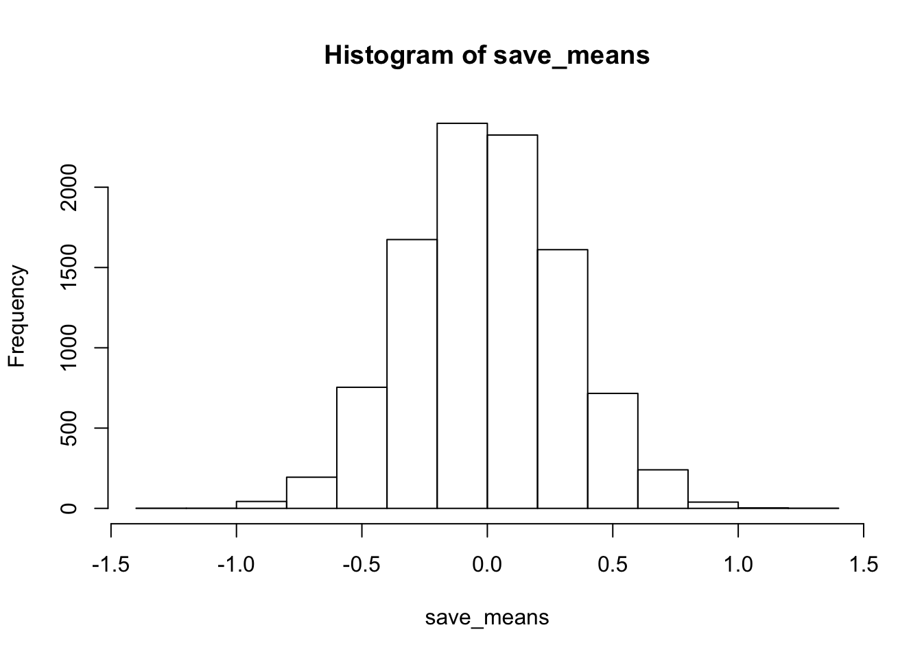
sd(save_means)## [1] 0.3115906mean(replicate(1000,mean(rnorm(10,0,1))))## [1] 0.001716855sd(replicate(1000,mean(rnorm(10,0,1))))## [1] 0.3176535hist(replicate(1000,sd(rnorm(10,0,1))))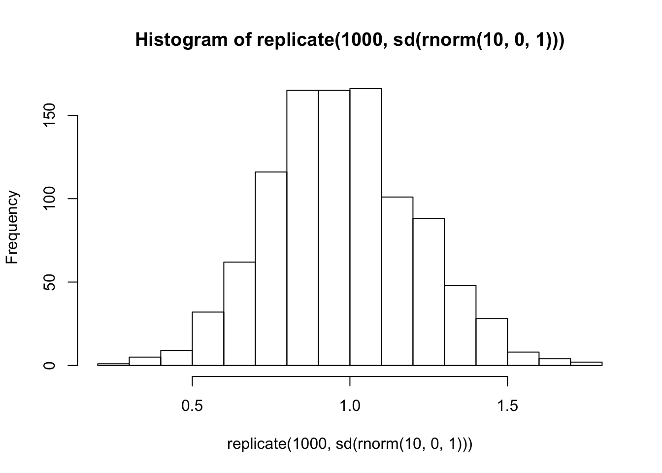
NULL
A <- rnorm(n=10,mean=0,sd=1)
B <- rnorm(n=10,mean=0,sd=1)
mean_diff <- mean(A-B)

mean_differ <- replicate(10000, mean(rnorm(n=10,mean=0,sd=1))-mean(rnorm(n=10,mean=0,sd=1)))
hist(mean_differ)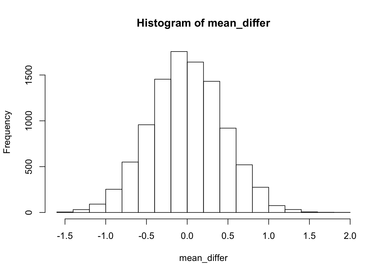
sort(mean_differ)[9500] # critical value## [1] 0.7476529TTEST
real_ps<- pt(q=c(.5,1,1.5,2,2.5), df=9)

t_s<- replicate(100,t.test(rnorm(10,0,1),mu=0)$statistic)

hist(t_s)
sim_ps<- c(length(t_s[t_s<.5])/100,
length(t_s[t_s<1])/100,
length(t_s[t_s<1.5])/100,
length(t_s[t_s<2])/100,
length(t_s[t_s<2.5])/100)

real_ps - sim_ps
## [1] 0.075464350 0.048281802 -0.013925328 -0.008276412 0.003069086sum(real_ps - sim_ps)## [1] 0.1046135CORRELATION
cor(rnorm(10,0,1),rnorm(10,0,1))## [1] 0.0456425hist(replicate(10000,cor(rnorm(10,0,1),rnorm(10,0,1))))
sim_rs <- replicate(10000,cor(rnorm(10,0,1),rnorm(10,0,1)))
sort(abs(sim_rs))[9500]
## [1] 0.6375356F-DISTRIBUTION
run_anova<- function(){
A <- rnorm(4,0,1)
B <- rnorm(4,0,1)
C <- rnorm(4,0,1)

conds<- rep(c("A","B","C"),each = 4)
DV <- c(A,B,C)
der <- data.frame(conds,DV)
sum_o <-summary(aov(DV~conds,der))
return(sum_o[[1]]$`F value`[1])
}

sim_fs<- replicate(10000,run_anova())

a.a<-sort(sim_fs)[9500]

a.b<- qf(.95,2,9)
04/01/19 More Papaja & Power Analysis
papaja manual
# Seed for random number generation
set.seed(42)
knitr::opts_chunk$set(cache.extra = knitr::rand_seed)
Methods
We report how we determined our sample size, all data exclusions (if any), all manipulations, and all measures in the study.
Participants
Material
Procedure
Data analysis
We used r cite_r(“r-references.bib”) for all our analyses.
Results
you can control sizing in the {r, fig.width, fig.height, out.height, out.width}
@R-base
a<- rnorm(100,0,1)
hist(a)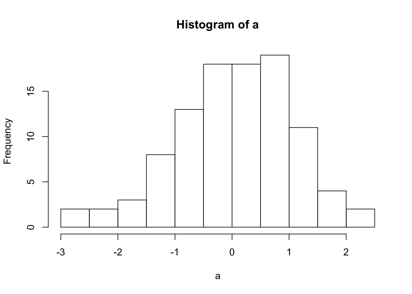
this figure is a histogram
a <- c(1,2,3)
sapply(a, FUN=function(x){
  paste(x, "a", sep = "")
})
## [1] "1a" "2a" "3a"Power Analysis:
Bold Claim: If you can’t simulate your data, you might not understand it very well.
This week on simulation shows you how to generate simulated data in R. There are many reasons to do this, including:
- Develop a deeper understanding of the assumptions behind statistical tests
- Sample-size planning and power-analysis
- Understand how real data ought to behave given the assumptions you are making about the data.
Null-hypothesis
In general, the null-hypothesis is the hypothesis that your experimental manipulation didn’t work. Or, the hypothesis of no differences.
We can simulate null-hypotheses in R for any experimental design. We do this in the following way:
- Use R to generate sample data in each condition of a design
- Make sure the sample data comes from the very same distribution for all conditions (ensure that there are no differences)
- Compute a test-statistic for each simulation, save it, then repeat to create the sampling distribution of the test statistic.
- The sampling distribution of the test-statistic is the null-distribution. We use it to set an alpha criterion, and then do hypothesis testing.
Null for a t-test
# samples A and B come from the same normal distribution
A <- rnorm(n=10,mean=10, sd=5)
B <- rnorm(n=10,mean=10, sd=5)
# the pvalue for this one pretend simulation
t.test(A,B,var.equal=TRUE)$p.value
## [1] 0.3711599# running the simulation
# everytime we run this function we do one simulated experiment and return the p-value
sim_null <- function(){
A <- rnorm(n=10,mean=10, sd=5)
B <- rnorm(n=10,mean=10, sd=5)
return(t.test(A,B,var.equal=TRUE)$p.value)
}
# use replicate to run the sim many times
outcomes <- replicate(1000,sim_null())
# plot the null-distribution of p-values
hist(outcomes)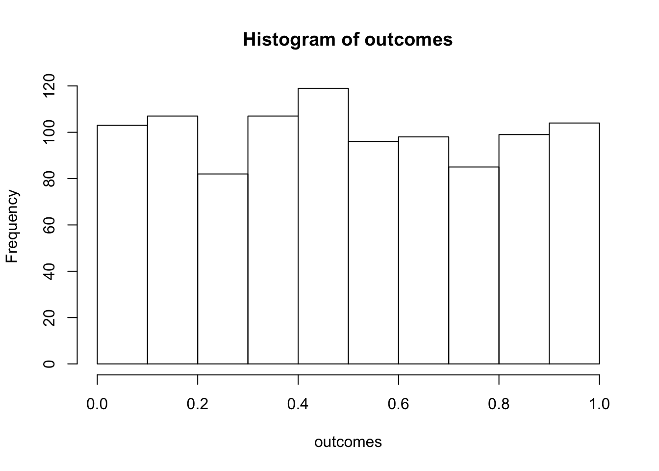
# proportion of simulated experiments had a p-value less than .05
length(outcomes[outcomes<.05])/1000
## [1] 0.046We ran the above simulation 1000 times. By definition, we should get approximately 5% of the simulations returning a p-value less than .05. If we increase the number of simulations, then we will get a more accurate answer that converges on 5% every time.
Alternative hypothesis
The very general alternative to the null hypothesis (no differences), is often called the alternative hypothesis: that the manipulation does cause a difference. More specifically, there are an infinite number of possible alternative hypotheses, each involving a difference of a specific size.
Consider this. How often will we find a p-value less than .05 if there was a mean difference of 5 between sample A and B. Let’s use all of the same parameters as before, except this time we sample from different distributions for A and B.
# make the mean for B 15 (5 more than A)
sim_alternative <- function(){
  A <- rnorm(n=10,mean=10, sd=5)
  B <- rnorm(n=10,mean=15, sd=5)
  return(t.test(A,B,var.equal=TRUE)$p.value)
}
# use replicate to run the sim many times
outcomes <- replicate(1000,sim_alternative())
# plot the distribution of p-values
hist(outcomes)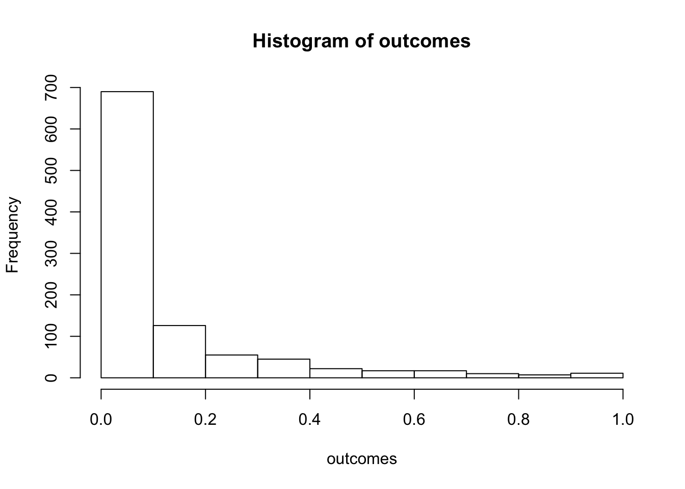
# proportion of simulated experiments had a p-value less than .05
length(outcomes[outcomes<.05])/1000
## [1] 0.537We programmed a mean difference of 5 between our sample for A and B, and we found p-values less than .05 a much higher proportion of the time. This is sensible, as there really was a difference between the samples (we put it there).
Power and Effect Size
Power: the probability of rejecting a null-hypothesis, given that there is a true effect of some size.
Effect-size: In general, it’s the assumed size of the difference. In the above example, we assumed a difference of 5, so the assumed effect-size was 5.
There are many other ways to define and measure effect-size. Perhaps the most common way is Cohen’s D. Cohen’s D expresses the mean difference in terms of standard deviation units. In the above example, both distributions had a standard deviation of 5. The mean for A was 10, and the mean for B was 15. Using Cohen’s D, the effect-size was 1. This is because 15 is 1 standard deviation away from 10 (the standard deviation is also 5).
When we calculated the proportion of simulations that returned a p-value less than .05, we found the power of the design to detect an effect-size of 1.
Power depends on three major things:
- Sample-size
- Effect-size
- Alpha-criterion
Power is a property of a design. The power of a design increases when sample-size increases. The power of a design increases when the actual true effect-size increases. The power of a design increases then the alpha criterion increases (e.g, going from .05 to .1, making it easier to reject the null).
Power analysis with R
There are many packages and functions for power analysis. Power analysis is important for planning a design. For example, you can determine how many subjects you need in order to have a high probability of detecting a true effect (of a particular size) if it is really there.
pwr package
Here is an example of using the pwr package to find the power for an independent sample t-test, with n=10, to detect an effect-size of 1. This answer is similar to our simulations answer. The simulation would converge on this answer if we increased the number of simulations.
library(pwr)
pwr.t.test(n=10,
           d=1,
           sig.level=.05,
           type="two.sample",
           alternative="two.sided")
##
## Two-sample t test power calculation
##
## n = 10
## d = 1
## sig.level = 0.05
## power = 0.5620066
## alternative = two.sided
##
## NOTE: n is number in *each* groupAs I mentioned there are many functions for directly computing power in R. Feel free to use them. In this class, we learn how to use simulation to conduct power analyses. This can be a redundant approach that is not necessary, given there are other functions we can use. Additionally, we will not get exact solutions (but approximate ones). Nevertheless, the existing power functions can be limited and may not apply to your design. The simulation approach can be extended to any design. Learning how to run the simulations will also improve your statistical sensibilities, and power calculations will become less of a black box.
Two more things before moving onto simulation: power-curves, and sample-size planning.
power-curves
A design’s power is in relation to the true effect-size. The same design has different levels of power to detect different sized effects. Let’s make a power curve to see the power of a t-test for independent samples (n=10) to detect a range of effect-sizes
effect_sizes <- seq(.1,2,.1)
power <- sapply(effect_sizes,
          FUN = function(x) {
            pwr.t.test(n=10,
            d=x,
            sig.level=.05,
            type="two.sample",
            alternative="two.sided")$power})
plot_df <- data.frame(effect_sizes,power)
library(ggplot2)
ggplot(plot_df, aes(x=effect_sizes,
                    y=power))+
  geom_point()+
  geom_line()
This power curve applies to all independent-sample t-tests with n=10. It is a property, or fact about those designs. Every design has it’s own power curve. The power curve shows us what should happen (on average), when the true state of the world involves effects of different sizes.
If you do not know the power-curve for your design, then you do not know how sensitive your design is for detecting effects of particular sizes. You might accidentally be using an under powered design, with only a very small chance of detecting an effect of a size you are interested in.
If you do know the power-curve for your design, you will be in a better position to plan your experiment, for example by modifying the number of subjects that you run.
Sample-size planning
Here is one way to plan for the number of subjects that you need to find an effect of interest.
- Establish a smallest effect-size of interest
- Create a curve showing the power of your design as a function of number of subjects to detect the smallest effect-size of interest.
It’s not clear how you establish a smallest effect-size of interest. But let’s say you are interested in detecting an effect of at least d = .2. This means that two conditions would differ by at least a .2 standard deviation shift. If you find something smaller than that, let’s say you wouldn’t care about it because it wouldn’t be big enough for you to care. How many subjects do you need to have a high powered design, one that would almost always reject the null-hypothesis?
This is for an independent samples t-test:
num_subjects <- seq(10,1000,10)
power <- sapply(num_subjects,
          FUN = function(x) {
            pwr.t.test(n=x,
            d=.2,
            sig.level=.05,
            type="two.sample",
            alternative="two.sided")$power})
plot_df <- data.frame(num_subjects,power)
library(ggplot2)
ggplot(plot_df, aes(x=num_subjects,
                    y=power))+
  geom_point()+
  geom_line()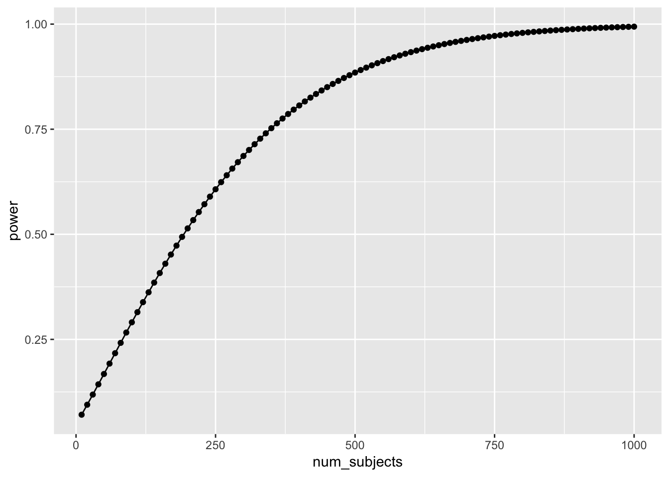
Well, it looks like you need many subjects to have high power. For example, if you want to detect the effect 95% of the time, you would need around 650 subjects. It’s worth doing this kind of analysis to see if your design checks out. You don’t want to waste your time running an experiment that is designed to fail (even when the true effect is real).
Simulation approach to power calculations
The simulation approach to power analysis involves these steps:
- Use R to sample numbers into each condition of any design.
- You can set the properties (e.g., n, mean, sd, kind of distribution etc.) of each sample in each condition, and mimic any type of expected pattern
- Analyze the simulated data to obtain a p-value (use any analysis appropriate to the design)
- Repeat many times, save the p-values
- Compute power by determining the proportion of simulated p-values that are less than your alpha criterion.
For all simulations, increasing number of simulations will improve the accuracy of your results. We will use 1000 simulations throughout. 10,000 would be better, but might take just a little bit longer.
Simulated power for a t-test
A power curve for n=10.
# function to run a simulated t-test
sim_power <- function(x){
  A <- rnorm(n=10,mean=0, sd=1)
  B <- rnorm(n=10,mean=(0+x), sd=1)
  return(t.test(A,B,var.equal=TRUE)$p.value)
}
# vector of effect sizes
effect_sizes <- seq(.1,2,.1)
# run simulation for each effect size 1000 times
power <- sapply(effect_sizes,
          FUN = function(x) {
            sims <- replicate(1000,sim_power(x))
            sim_power <- length(sims[sims<.05])/length(sims)
            return(sim_power)})
# combine into dataframe
plot_df <- data.frame(effect_sizes,power)
# plot the power curve
ggplot(plot_df, aes(x=effect_sizes,
                    y=power))+
  geom_point()+
  geom_line()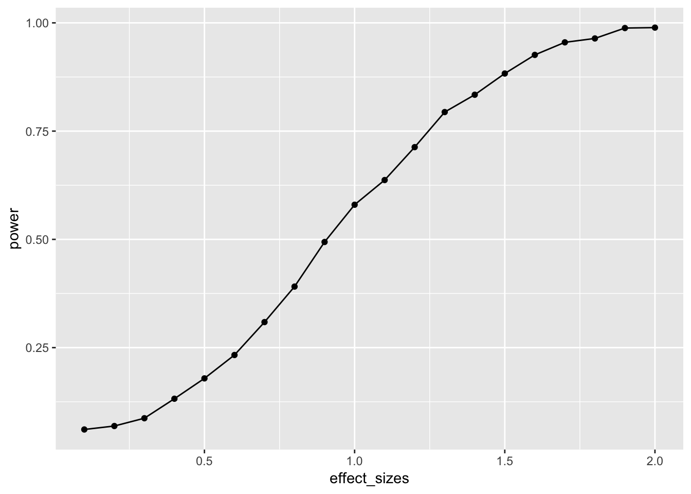
In this case, there is no obvious benefit to computing the power-curve by simulation. The answer we get is similar to the answer we got before using the pwr package, but our simulation answer is more noisy. Why bother the simulation?
One answer to the why bother question is that you can simulate deeper aspects of the design and get more refined answers without having to work through the math.
Simulating cell-size
Many experimental designs involve multiple measurements, or trials, for each subject in each condition. How many trials should we require for each subject in each condition? Traditional power analysis doesn’t make it easy to answer this question. However, the power of a design will depend not only on the number subjects, but also the number trials used to estimate the mean for each subject in each condition.
Consider a simple Stroop experiment. The researcher is interested in measuring a Stroop effect of at least d=.1 (e.g., the difference between mean congruent trials is .1 standard deviations smaller than mean incongruent trials). How many subjects are required? And, how many trials should each subject perform in the congruent and incongruent conditions? Let’s use simulation to find out.
# function to run a simulated t-test
# nsubs sets number of subjects
# ntrials to change number of trials
# d sets effect size
# this is a paired sample test to model Stroop
sim_power <- function(nsubs,ntrials,d){
  A <- replicate(nsubs,mean(rnorm(n=ntrials,mean=0, sd=1)))
  B <- replicate(nsubs,mean(rnorm(n=ntrials,mean=d, sd=1)))
  return(t.test(A,B,paired=TRUE)$p.value)
}
# vectors for number of subjects and trials
n_subs_vector <- c(10,20,30,50)
n_trials_vector <- c(10,20,30,50,100)
# a loop to run all simulations
power <- c()
subjects <- c()
trials <- c()
i <- 0 # use this as a counter for indexing
for(s in n_subs_vector){
  for(t in n_trials_vector){
    i <- i+1
    sims <- replicate(1000,sim_power(s,t,.1))
    power[i] <- length(sims[sims<.05])/length(sims)
    subjects[i] <- s
    trials[i] <- t
  }
}
# combine into dataframe
plot_df <- data.frame(power,subjects,trials)
# plot the power curve
ggplot(plot_df, aes(x=subjects,
                    y=power,
                    group=trials,
                    color=trials))+
  geom_point()+
  geom_line()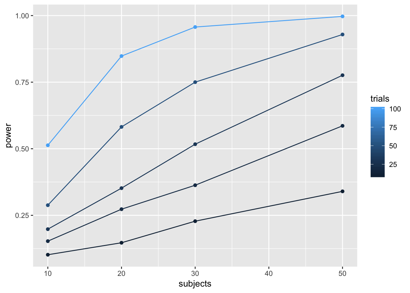
# a vectorized version of the loop
# run simulation for each effect size 1000 times
# power <- outer(n_subs_vector,
#                n_trials_vector,
#                FUN = Vectorize(function(x,y) {
#                   sims <- replicate(100,sim_power(x,y))
#                   sim_power <- length(sims[sims<.05])/length(sims)
#                   return(sim_power)
#                }))
To my eye, it looks like 30 subjects with 100 trials in each condition would give you a very high power to find a Stroop effect of d=.1.
One-Way ANOVA
Let’s extend our simulation based approach to the one-way ANOVA. Let’s assume a between-subjects design, with one factor that has four levels: A, B, C, and D. There will be 20 subjects in each group. What is the power curve for this design to detect effects of various size? Immediately, the situation becomes complicated, there are numerous ways that the means for A, B, C, and D could vary. Let’s assume the simplest case, three of them are the same, and one of them is different by some amount of standard deviations. We will compute the main effect, and report the proportion of significant experiments as we increase the effect size for the fourth group.
# function to run a simulated t-test
sim_power_anova <- function(x){
  A <- rnorm(n=20,mean=0, sd=1)
  B <- rnorm(n=20,mean=0, sd=1)
  C <- rnorm(n=20,mean=0, sd=1)
  D <- rnorm(n=20,mean=(0+x), sd=1)
  df <- data.frame(condition = as.factor(rep(c("A","B","C","D"),each=20)),
                   DV = c(A,B,C,D))
  aov_results <- summary(aov(DV~condition,df))
  #return the pvalue
  return(aov_results[[1]]$`Pr(>F)`[1])
}
# vector of effect sizes
effect_sizes <- seq(.1,2,.1)
# run simulation for each effect size 1000 times
power <- sapply(effect_sizes,
          FUN = function(x) {
            sims <- replicate(1000,sim_power_anova(x))
            sim_power <- length(sims[sims<.05])/length(sims)
            return(sim_power)})
# combine into dataframe
plot_df <- data.frame(effect_sizes,power)
# plot the power curve
ggplot(plot_df, aes(x=effect_sizes,
                    y=power))+
  geom_point()+
  geom_line()
It looks like this design (1 factor, between-subjects, 20 subjects per group) has high power to detect an effect of d=1, specifically when one of the groups differs from the others by d=1.
However, most effects in psychology are smalls, d=.2 is very common. How, many subjects does this design require to have high power (let’s say above .95, although most people use .8) to detect that small effect?
sim_power_anova <- function(x){
  A <- rnorm(n=x,mean=0, sd=1)
  B <- rnorm(n=x,mean=0, sd=1)
  C <- rnorm(n=x,mean=0, sd=1)
  D <- rnorm(n=x,mean=.2, sd=1)
  df <- data.frame(condition = as.factor(rep(c("A","B","C","D"),each=x)),
                   DV = c(A,B,C,D))
  aov_results <- summary(aov(DV~condition,df))
  #return the pvalue
  return(aov_results[[1]]$`Pr(>F)`[1])
}
# vector of effect sizes
subjects <- seq(10,1000,50)
# run simulation for each effect size 1000 times
power <- sapply(subjects,
          FUN = function(x) {
            sims <- replicate(1000,sim_power_anova(x))
            sim_power <- length(sims[sims<.05])/length(sims)
            return(sim_power)})
# combine into dataframe
plot_df <- data.frame(subjects,power)
# plot the power curve
ggplot(plot_df, aes(x=subjects,
                    y=power))+
  geom_point()+
  geom_line()
The simulations suggests we need about 560 subjects in each group to have power .95 to detect the effect (d=.2). That’s a total of 2240 subjects. Reality can be surprising when it comes to power analysis. It is better to be surprised about your design before you run your experiment, not after.
Closing thoughts
The simulation approach is powerful and flexible. It can be applied whenever you can formalize your assumptions about the data. And, your simulations can be highly customized to account for all kinds of nuances, like different numbers of subjects, different distributions, assumptions about noise, etc. If you are wondering what your design can do, maybe you should simulate it.
More example(s)
As I find time I will try to add more examples here, especially out of the box examples to illustrate how simulation can be applied.
Correlation between traits and behavior
A common research strategy is to measure putative correlations between people’s traits and their behavior. For example, a researcher might prepare a questionnaire with several questions. Perhaps the questions are about their political views, or about their life satisfaction, or anything else. The research might ask some group of people to answer the questions, and to also perform some task. At the end of the experiment, they might ask if different kinds of people (measured by the questionnaire) perform differently on the behavioral measure. For example, we might have people answer several questions about their openness to new experiences, we might also measure their performance on a working memory task. A research question might be, do people who are more open to experience perform better on a working memory task? The answer would lie in a correlation between the answers on the questions, and the performance on the task. Let’s simulate this kind of situation, say for 20 subjects. Each subject answers 20 questions, and they perform a behavioral task. At the end of the experiment, we correlate the answers on each question, with the performance on the task. What kind of correlations would we expect by chance alone? Let’s say the participants are all random robots. They answer each question randomly, and their performance on the behavioral task is sampled randomly from some normal distribution. If everything is random, shouldn’t we expect to find no correlations?
Details:
Let’s assume that each question involves a likert scale from 1 to 7. Each person randomly picks a number from 1 to 7 for each question. Let’s assume performance on the behavioral task is sampled from a normal distribution with mean = 0, and sd = 1.
# get 20 random answers for all 20 subjects and 20 questions
# columns will be individual subjects 1 to 20
# rows will be questions 1 to 20
questionnaire <- matrix(sample(1:7,20*20, replace=TRUE),ncol=20)
# get 20 measures of performance on behavioral task
behavioral_task <- rnorm(20,0,1)
# correlate behavior with each question
save_correlations <-c()
for(i in 1:20){
  save_correlations[i] <- cor(behavioral_task,questionnaire[i,])
}
# show histogram of 20 correlations
hist(save_correlations)
The histogram shows that a range of correlations between individual questions and behavior can emerge just by chance alone. If you run the above code a few times, you will see that the histogram changes a bit because of random chance.
Oftentimes researchers might not know which question on the questionnaire is the best question. That is, the one that best correlates with behavior. Consider a researcher who computes all of the correlations between each question and behavior, and then chooses the question with highest correlation (positive or negative) as the best question. After all, it has the highest correlation. After choosing this question, they might suggest that behavior is strongly correlated with how people answer this question.
Let’s try to find out by simulation what kinds of large correlations can occur just by chance alone. We will run the above many times, and each time we will save the absolute value of the largest correlation between a question and behavior. Just how large can these correlations be by chance alone?
save_max <- c()
for( j in 1:10000){
  questionnaire <- matrix(sample(1:7,20*20, replace=TRUE),ncol=20)
  behavioral_task <- rnorm(20,0,1)

  save_correlations <-c()
  for(i in 1:20){
    save_correlations[i] <- cor(behavioral_task,questionnaire[i,])
  }
  save_max[j] <- max(abs(save_correlations))
}
hist(save_max)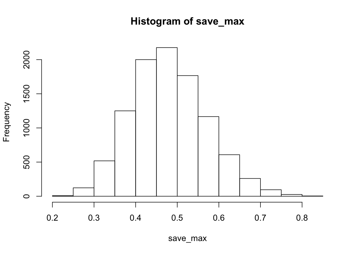
The simulation shows that chance alone in this situation can produce very large correlations, as large as .8 or .9 (although not very often).
The situation changes somewhat if many more subjects are run. Let’s do the same as above, but run 200 subjects, rather than 20.
save_max <- c()
for( j in 1:10000){
  questionnaire <- matrix(sample(1:7,200*20, replace=TRUE),ncol=200)
  behavioral_task <- rnorm(200,0,1)

  save_correlations <-c()
  for(i in 1:20){
    save_correlations[i] <- cor(behavioral_task,questionnaire[i,])
  }
  save_max[j] <- max(abs(save_correlations))
}
hist(save_max)
Now, chance doesn’t do much better than .25.
04/08/19 Shiny Web Apps
first main chunk: lay out the website, where buttons go & layout ui = user interface “shiny widgets” = button types & etc i.e. sliderinput (name of thing,) fluid page = shiny function for setting up webpages, you can add a title under it under it is a sidebar layout and a main bar panel
2nd part of the app: server (the R side of the app)
https://crumplab.github.io/psyc7709/Presentations/Shiny_tutorial.html
04/15/19 More Shiny and Optimization
Memory management
When you create objects in R, you are assigning part of your computer’s memory to represent the parts of the object. Generally speaking, your ability to create objects in R is limited by the memory of your computer. Additionally, the process of representing your object in memory takes time. So, memory management involves understanding how to efficiently represent information in memory.
The size of an object in memory depends on object class
# numeric by default
a <- rep(0,1000)
object.size(a)
## 8048 bytes# as.character
a <- as.character(rep(0,1000))
object.size(a)## 8104 bytes# as.integer
a <- as.integer(rep(0,1000))
object.size(a)## 4048 bytes# as.double
a <- as.double(rep(0,1000))
object.size(a)## 8048 bytesMatrices and data frames
b <- matrix(0,ncol=10,nrow=100)
object.size(b)
## 8216 bytesc <- as.data.frame(matrix(0,ncol=10,nrow=100))
object.size(c)## 9904 bytesRprofvis
Rprof(tmp <- tempfile())

a <- matrix(0,nrow=2,ncol=1000)
for(i in 1:1000){
  a <- rbind(a,rnorm(1000,0,1))
}

Rprof()
summaryRprof(tmp)
## $by.self
## self.time self.pct total.time total.pct
## "rbind" 7.98 92.79 8.00 93.02
## "eval" 0.60 6.98 8.60 100.00
## "rnorm" 0.02 0.23 0.02 0.23
##
## $by.total
## total.time total.pct self.time self.pct
## "eval" 8.60 100.00 0.60 6.98
## "block_exec" 8.60 100.00 0.00 0.00
## "call_block" 8.60 100.00 0.00 0.00
## "evaluate_call" 8.60 100.00 0.00 0.00
## "evaluate::evaluate" 8.60 100.00 0.00 0.00
## "evaluate" 8.60 100.00 0.00 0.00
## "FUN" 8.60 100.00 0.00 0.00
## "generator$render" 8.60 100.00 0.00 0.00
## "handle" 8.60 100.00 0.00 0.00
## "in_dir" 8.60 100.00 0.00 0.00
## "knitr::knit" 8.60 100.00 0.00 0.00
## "lapply" 8.60 100.00 0.00 0.00
## "process_file" 8.60 100.00 0.00 0.00
## "process_group.block" 8.60 100.00 0.00 0.00
## "process_group" 8.60 100.00 0.00 0.00
## "render_one" 8.60 100.00 0.00 0.00
## "rmarkdown::render_site" 8.60 100.00 0.00 0.00
## "rmarkdown::render" 8.60 100.00 0.00 0.00
## "sapply" 8.60 100.00 0.00 0.00
## "suppressMessages" 8.60 100.00 0.00 0.00
## "timing_fn" 8.60 100.00 0.00 0.00
## "withCallingHandlers" 8.60 100.00 0.00 0.00
## "withVisible" 8.60 100.00 0.00 0.00
## "rbind" 8.00 93.02 7.98 92.79
## "rnorm" 0.02 0.23 0.02 0.23
##
## $sample.interval
## [1] 0.02
##
## $sampling.time
## [1] 8.6Rprof(tmp <- tempfile())
a <- matrix(0,nrow=1002,ncol=1000)
for(i in 3:1002){
a[i,] <- rnorm(1000,0,1)
}
Rprof()
summaryRprof(tmp)## $by.self
## self.time self.pct total.time total.pct
## "rnorm" 0.14 87.5 0.14 87.5
## "eval" 0.02 12.5 0.16 100.0
##
## $by.total
## total.time total.pct self.time self.pct
## "eval" 0.16 100.0 0.02 12.5
## "block_exec" 0.16 100.0 0.00 0.0
## "call_block" 0.16 100.0 0.00 0.0
## "evaluate_call" 0.16 100.0 0.00 0.0
## "evaluate::evaluate" 0.16 100.0 0.00 0.0
## "evaluate" 0.16 100.0 0.00 0.0
## "FUN" 0.16 100.0 0.00 0.0
## "generator$render" 0.16 100.0 0.00 0.0
## "handle" 0.16 100.0 0.00 0.0
## "in_dir" 0.16 100.0 0.00 0.0
## "knitr::knit" 0.16 100.0 0.00 0.0
## "lapply" 0.16 100.0 0.00 0.0
## "process_file" 0.16 100.0 0.00 0.0
## "process_group.block" 0.16 100.0 0.00 0.0
## "process_group" 0.16 100.0 0.00 0.0
## "render_one" 0.16 100.0 0.00 0.0
## "rmarkdown::render_site" 0.16 100.0 0.00 0.0
## "rmarkdown::render" 0.16 100.0 0.00 0.0
## "sapply" 0.16 100.0 0.00 0.0
## "suppressMessages" 0.16 100.0 0.00 0.0
## "timing_fn" 0.16 100.0 0.00 0.0
## "withCallingHandlers" 0.16 100.0 0.00 0.0
## "withVisible" 0.16 100.0 0.00 0.0
## "rnorm" 0.14 87.5 0.14 87.5
##
## $sample.interval
## [1] 0.02
##
## $sampling.time
## [1] 0.1605/06/19 Bookdown & Final Presentation
link on page by having name you want displayed in brackets followed by parantheses with the link
Bookdown- save chapters w file name in number order Index has “prerequisites” Bookdown themes online will give you different styles for the book