Solving Problems
Introduction
This is the heart of my online journal where i will be working through problems provided by the instructor as well as practicing code on my own.
Practice
first <- c("ja","we", "uj", "wx", "he")
last <- c("kjf", "sGsd", "asfhb", "jasd", "sdkjfg")
age <- c(34,645,23,85,1234)

sd<- list(First=first, Last=last, C=age)
names(sd)[3]<- "DOB"
Find the longest word
x<- "a dog went for a walk to the circuis"

#first<- strsplit(x, split = " ")
#first[[1]][1]

longest<- function(x)
for (j in 1:length(x))
  x<-unlist((strsplit(x, split = " ")))
  x<-tail(sort(x))
Histogram
samples<- rnorm(100, mean=50, sd=5)
hist(samples)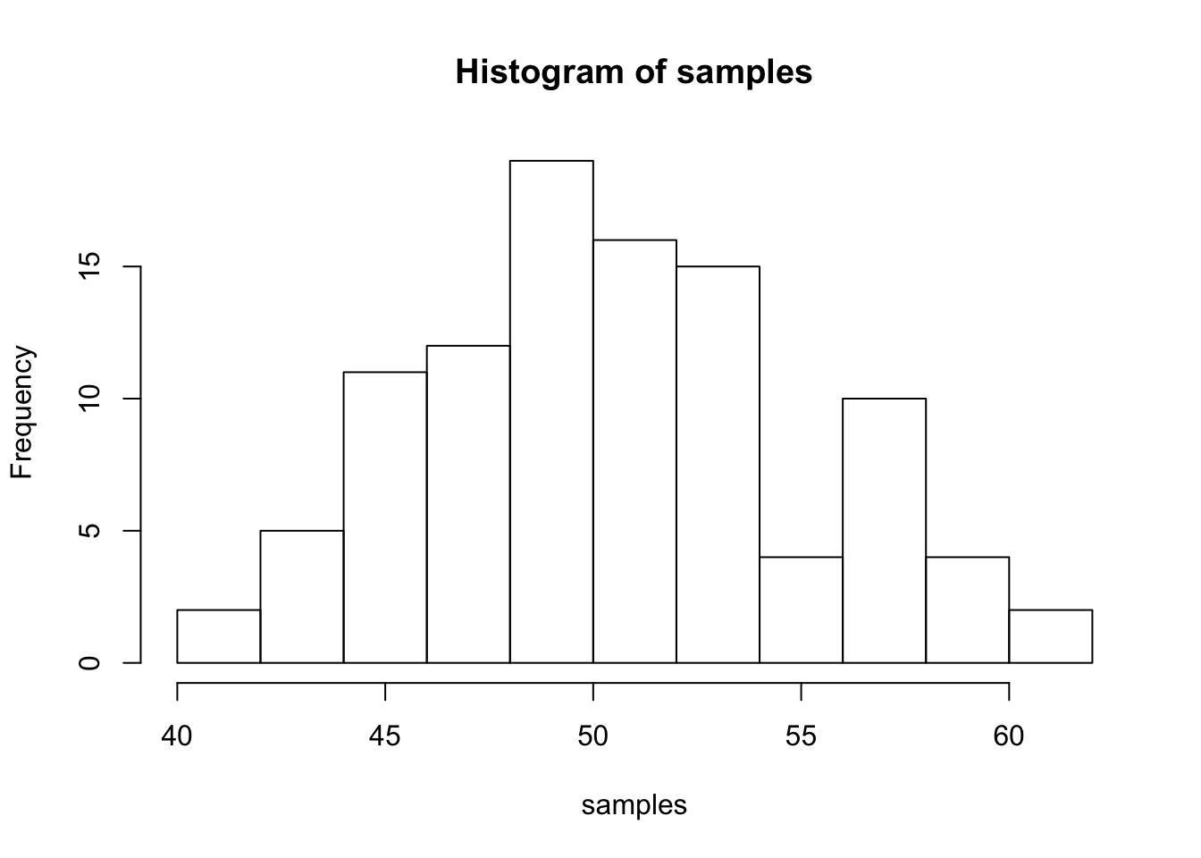
Rent of $750 for 12 months added using a loop
b<-length(12)
for(j in 1:12){
  b[j]<-750
}
c<- sum(b)
print(c)
## [1] 9000Plot sensitivity curves for S,M & L cones
Slen<- seq(320,500,10)
Mlen<- seq(440,650,10)
Llen<- seq(480,680,10)

Smean<- 420
Mmean<- 530
Lmean<- 560

Sx<-dnorm(Slen,Smean,1)

plot(Slen,Sx,type="n", xlab ="Wavelength", ylab = "Sensitivity", axes = TRUE)
Easier Problems
- Do simple math with numbers, addition, subtraction, multiplication and division
2+3## [1] 512-7## [1] 55*3## [1] 1525/2.5## [1] 10- Put numbers into variables, do simple math on the variables
x<- 22
y<- 4
z<- 6
x-y
## [1] 18y*z## [1] 24- Write a code that will place the numbers 1 to 100 separately into a variable using for loop. Then again using the seq function.
a<- length(100)
for(i in 1:100){
  a[i]<- i
}
d<-seq(1,100,1)
print(d)## [1] 1 2 3 4 5 6 7 8 9 10 11 12 13 14 15 16 17
## [18] 18 19 20 21 22 23 24 25 26 27 28 29 30 31 32 33 34
## [35] 35 36 37 38 39 40 41 42 43 44 45 46 47 48 49 50 51
## [52] 52 53 54 55 56 57 58 59 60 61 62 63 64 65 66 67 68
## [69] 69 70 71 72 73 74 75 76 77 78 79 80 81 82 83 84 85
## [86] 86 87 88 89 90 91 92 93 94 95 96 97 98 99 100- Find the sum of all the integer numbers from 1 to 100.
print(sum(d))## [1] 5050- Write a function to find the sum of all integers between any two values.
sum_of_integers<-function(e,f){
  return (sum(seq(e,f,1)))
}


sum_of_integers(8,99)
## [1] 4922- List all of the odd numbers from 1 to 100.
odd<-seq(1,100,2)
print(odd)
## [1] 1 3 5 7 9 11 13 15 17 19 21 23 25 27 29 31 33 35 37 39 41 43 45
## [24] 47 49 51 53 55 57 59 61 63 65 67 69 71 73 75 77 79 81 83 85 87 89 91
## [47] 93 95 97 99- List all of the prime numbers from 1 to 1000.
for (k in 2:1000) {
  prime<- TRUE

  for (x in 2:(k-1)){
    if(k %% x==0){
      prime<- FALSE

    }
  }
  if(prime == TRUE){
    print(k)
  }
  }
## [1] 3
## [1] 5
## [1] 7
## [1] 11
## [1] 13
## [1] 17
## [1] 19
## [1] 23
## [1] 29
## [1] 31
## [1] 37
## [1] 41
## [1] 43
## [1] 47
## [1] 53
## [1] 59
## [1] 61
## [1] 67
## [1] 71
## [1] 73
## [1] 79
## [1] 83
## [1] 89
## [1] 97
## [1] 101
## [1] 103
## [1] 107
## [1] 109
## [1] 113
## [1] 127
## [1] 131
## [1] 137
## [1] 139
## [1] 149
## [1] 151
## [1] 157
## [1] 163
## [1] 167
## [1] 173
## [1] 179
## [1] 181
## [1] 191
## [1] 193
## [1] 197
## [1] 199
## [1] 211
## [1] 223
## [1] 227
## [1] 229
## [1] 233
## [1] 239
## [1] 241
## [1] 251
## [1] 257
## [1] 263
## [1] 269
## [1] 271
## [1] 277
## [1] 281
## [1] 283
## [1] 293
## [1] 307
## [1] 311
## [1] 313
## [1] 317
## [1] 331
## [1] 337
## [1] 347
## [1] 349
## [1] 353
## [1] 359
## [1] 367
## [1] 373
## [1] 379
## [1] 383
## [1] 389
## [1] 397
## [1] 401
## [1] 409
## [1] 419
## [1] 421
## [1] 431
## [1] 433
## [1] 439
## [1] 443
## [1] 449
## [1] 457
## [1] 461
## [1] 463
## [1] 467
## [1] 479
## [1] 487
## [1] 491
## [1] 499
## [1] 503
## [1] 509
## [1] 521
## [1] 523
## [1] 541
## [1] 547
## [1] 557
## [1] 563
## [1] 569
## [1] 571
## [1] 577
## [1] 587
## [1] 593
## [1] 599
## [1] 601
## [1] 607
## [1] 613
## [1] 617
## [1] 619
## [1] 631
## [1] 641
## [1] 643
## [1] 647
## [1] 653
## [1] 659
## [1] 661
## [1] 673
## [1] 677
## [1] 683
## [1] 691
## [1] 701
## [1] 709
## [1] 719
## [1] 727
## [1] 733
## [1] 739
## [1] 743
## [1] 751
## [1] 757
## [1] 761
## [1] 769
## [1] 773
## [1] 787
## [1] 797
## [1] 809
## [1] 811
## [1] 821
## [1] 823
## [1] 827
## [1] 829
## [1] 839
## [1] 853
## [1] 857
## [1] 859
## [1] 863
## [1] 877
## [1] 881
## [1] 883
## [1] 887
## [1] 907
## [1] 911
## [1] 919
## [1] 929
## [1] 937
## [1] 941
## [1] 947
## [1] 953
## [1] 967
## [1] 971
## [1] 977
## [1] 983
## [1] 991
## [1] 997pr<- data.frame(1:1000)
pr[pr!%% pr == 0]- Generate 100 random numbers.
randnum<- sample(100)
randnum
## [1] 23 99 33 49 13 66 81 90 18 70 96 1 83 9 17 54 11
## [18] 2 86 16 51 85 22 10 12 60 79 31 27 80 56 67 62 53
## [35] 52 73 3 39 37 40 43 42 14 91 34 58 35 69 77 47 57
## [52] 44 4 71 36 94 64 48 55 78 26 28 29 15 97 41 6 19
## [69] 89 46 100 59 98 93 45 63 87 30 74 72 20 5 95 32 65
## [86] 75 24 50 7 38 68 92 82 21 76 25 8 61 84 88- Generate 100 random numbers within a specific range.
randrange<- sample(1:25,100,replace=T)
randrange
## [1] 7 13 21 20 8 4 9 5 13 19 9 11 15 11 13 8 21 9 1 19 19 19 18
## [24] 13 21 13 24 11 20 19 18 22 14 5 10 21 4 25 4 3 8 12 10 1 6 4
## [47] 3 8 9 7 7 8 18 19 5 14 9 6 15 4 2 10 12 13 16 21 3 25 8
## [70] 8 17 6 3 12 20 14 11 12 1 15 19 14 15 5 8 9 9 5 1 9 15 3
## [93] 12 2 7 11 16 22 6 5- Write your own functions to give descriptive statistics for a vector variable storing multiple numbers. Write functions for the following without using R intrinsics: mean, mode, median, range, standard deviation.
Average function
vector <- c(3,4,3,2,5,8,12)
aver<-function(avg_vec){
  avg_vec<- (sum(vector))/length(vector)
  return(avg_vec)
}
aver(vector)
## [1] 5.285714Mode
mode<-function(mode_vec){
  mode_vec<- sort(table(mode_vec))
  return(which.max(mode_vec))

}
de <- c(4,4,5,7,2,2,1)
mode(de)
## 2
## 4# ?Median
median<-function(w){
  med<- sort(w) #maybe make it proportion?
  n<- (length(med) +1 /2)
     return(med[n])

}
med_vec <- c(3,9,4,2,6,8)
median(med_vec)
## [1] 9Mean (take 2)
vector <- c(3,4,3,2,5,8,12)
mean<-function(x){
  return((sum(x))/length(x))
}
mean(vector)
## [1] 5.285714Range
range<-function(x){
  sort(x)
  return((max(x))-min(x))
}
Standard Deviation
std<-function(x){
  return(sqrt((sum((x-mean(x))^2))/length(x)))
}- Count the number of characters in a string variable.
nchar("ejsbfn;sl")## [1] 9- Count the number of words in a string variable.
d<- "i was going to the bank when i saw a bird"
sapply(strsplit(d," "),length)
## [1] 11- Count the number of sentences in a string variable.
e<- "sdsdf. gdg. ragrg. sgdthrtngf. gnfghnn"
#stuck- Count the number of times a specific character occurs in a string variable.
abc <- "rgjbndvlnkvb"
table(abc)
## abc
## rgjbndvlnkvb
## 1#not right- Do a logical test to see if one word is found within the text of another string variable.
h<-"bdaj jhsf dkjn fcjb fjkb"
h<-strsplit(h,split = " ")
h
## [[1]]
## [1] "bdaj" "jhsf" "dkjn" "fcjb" "fjkb""dkjn" %in% h## [1] FALSE#not working- Put the current computer time in milliseconds into a variable.
now<- Sys.time()
print(as.numeric(now))
## [1] 1556559371#?- Measure how long a piece of code takes to run by measuring the time before the code is run, and after the code is run, and taking the difference to find the total time.
?Sys.time- Read a .txt file or .csv file into a variable.
as.data.frame(read.table(flatfile_grades,header=TRUE,sep=","))Output the contents of a variable to a .txt file.
Create a variable that stores a 20x20 matrix of random numbers.
zyx <- matrix(0,nrow=20,ncol=20)- Output any matrix to a txt file using commas or tabs to separate column values, and new lines to separate row values.
Harder Problems
- The FizzBuzz Problem. List the numbers from 1 to 100 with the following constraints. If the number can be divided by three evenly, then print Fizz instead of the number. If the number can be divided by five evenly, then print Buzz instead of the number. Finally, if the number can be divided by three and five evenly, then print FizzBuzz instead of the number.
num <- 1:100
for (fb in num) {

  if((num[fb]%%3==0) && (num[fb]%%5==0)){
        print("FizzBuzz")
        next()
  }

  if (num[fb]%%3==0){
      print("Fizz")
      next()
  }

#      ifelse((num[fb]%%3==0) && (num[fb]%%5==0),1,0)
  #        print("FizzBuzz")


 if (num[fb]%%5==0){
   print("Buzz")
   next()
}

   else{
     (print(num[fb]))
   }
 }
## [1] 1
## [1] 2
## [1] "Fizz"
## [1] 4
## [1] "Buzz"
## [1] "Fizz"
## [1] 7
## [1] 8
## [1] "Fizz"
## [1] "Buzz"
## [1] 11
## [1] "Fizz"
## [1] 13
## [1] 14
## [1] "FizzBuzz"
## [1] 16
## [1] 17
## [1] "Fizz"
## [1] 19
## [1] "Buzz"
## [1] "Fizz"
## [1] 22
## [1] 23
## [1] "Fizz"
## [1] "Buzz"
## [1] 26
## [1] "Fizz"
## [1] 28
## [1] 29
## [1] "FizzBuzz"
## [1] 31
## [1] 32
## [1] "Fizz"
## [1] 34
## [1] "Buzz"
## [1] "Fizz"
## [1] 37
## [1] 38
## [1] "Fizz"
## [1] "Buzz"
## [1] 41
## [1] "Fizz"
## [1] 43
## [1] 44
## [1] "FizzBuzz"
## [1] 46
## [1] 47
## [1] "Fizz"
## [1] 49
## [1] "Buzz"
## [1] "Fizz"
## [1] 52
## [1] 53
## [1] "Fizz"
## [1] "Buzz"
## [1] 56
## [1] "Fizz"
## [1] 58
## [1] 59
## [1] "FizzBuzz"
## [1] 61
## [1] 62
## [1] "Fizz"
## [1] 64
## [1] "Buzz"
## [1] "Fizz"
## [1] 67
## [1] 68
## [1] "Fizz"
## [1] "Buzz"
## [1] 71
## [1] "Fizz"
## [1] 73
## [1] 74
## [1] "FizzBuzz"
## [1] 76
## [1] 77
## [1] "Fizz"
## [1] 79
## [1] "Buzz"
## [1] "Fizz"
## [1] 82
## [1] 83
## [1] "Fizz"
## [1] "Buzz"
## [1] 86
## [1] "Fizz"
## [1] 88
## [1] 89
## [1] "FizzBuzz"
## [1] 91
## [1] 92
## [1] "Fizz"
## [1] 94
## [1] "Buzz"
## [1] "Fizz"
## [1] 97
## [1] 98
## [1] "Fizz"
## [1] "Buzz"- Frequency Counts Take text as input, and be able to produce a table that shows the counts for each character in the text. This problem is related to the earlier easy problem asking you to count the number of times that a single letter appears in a text. The slightly harder problem is the more general version: count the frequencies of all unique characters in a text.
bah<-"hello and welcome to R"
b<-unique(unlist(strsplit(bah,split="")))
#bb<-data.frame(b,)
print(b)
## [1] "h" "e" "l" "o" " " "a" "n" "d" "w" "c" "m" "t" "R"- Test the Random Number Generator Test the random number generator for a flat distribution. Generate a few million random numbers between 0 and 100. Count the number of 0s, 1s, 2s, 3s, etc. all the way up to 100. Look at the counts for each of the numbers and determine if they are relatively equal. For example, you could plot the counts in Excel to make a histogram. If all of the bars are close to being flat, then each number had an equal chance of being selected, and the random number generator is working without bias.
milli <-floor(runif(5000000, 0,100))
table(milli)
## milli
## 0 1 2 3 4 5 6 7 8 9 10 11
## 50127 50077 50026 49843 50421 49948 50390 49889 50308 49900 49969 49740
## 12 13 14 15 16 17 18 19 20 21 22 23
## 49814 49866 49844 49857 50013 50207 50144 49976 49739 50101 50032 49875
## 24 25 26 27 28 29 30 31 32 33 34 35
## 50018 49526 50206 50253 50048 49972 49879 49959 49909 49944 49835 49949
## 36 37 38 39 40 41 42 43 44 45 46 47
## 50163 50271 49963 49962 50025 50339 50190 49807 49583 50002 50010 49877
## 48 49 50 51 52 53 54 55 56 57 58 59
## 50068 49978 50208 49602 50431 49902 50005 49742 50253 49933 49949 49768
## 60 61 62 63 64 65 66 67 68 69 70 71
## 49412 49971 50139 50060 50008 50386 50220 49985 50119 49695 50135 49954
## 72 73 74 75 76 77 78 79 80 81 82 83
## 50061 50220 49761 50381 49603 50376 49943 49767 50048 49860 50214 49975
## 84 85 86 87 88 89 90 91 92 93 94 95
## 50370 49931 50210 49790 50084 49961 49953 49636 50560 50204 49793 49753
## 96 97 98 99
## 49920 49873 50364 49670hist(milli)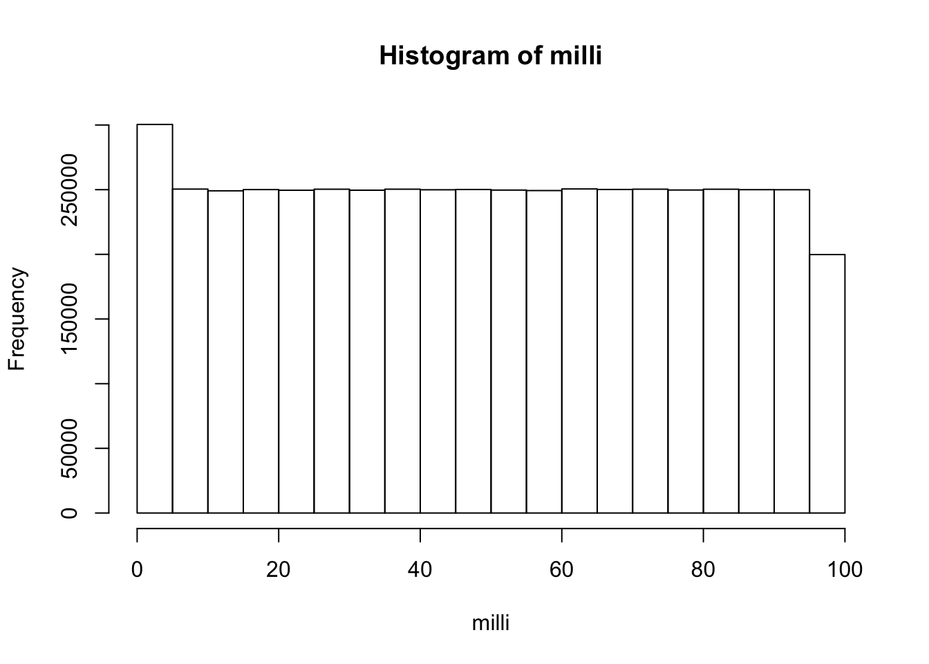
- Create a multiplication table Generate a matrix for a multiplication table. For example, the labels for the columns could be the numbers 1 to 10, and the labels for the rows could be the numbers 1 to 10. The contents of each of the cells in the matrix should be correct answer for multiplying the column value by the row value.
r<-1:10
c<-1:10
matrix(r*c, nrow = 10, ncol = 10, byrow = TRUE )
## [,1] [,2] [,3] [,4] [,5] [,6] [,7] [,8] [,9] [,10]
## [1,] 1 4 9 16 25 36 49 64 81 100
## [2,] 1 4 9 16 25 36 49 64 81 100
## [3,] 1 4 9 16 25 36 49 64 81 100
## [4,] 1 4 9 16 25 36 49 64 81 100
## [5,] 1 4 9 16 25 36 49 64 81 100
## [6,] 1 4 9 16 25 36 49 64 81 100
## [7,] 1 4 9 16 25 36 49 64 81 100
## [8,] 1 4 9 16 25 36 49 64 81 100
## [9,] 1 4 9 16 25 36 49 64 81 100
## [10,] 1 4 9 16 25 36 49 64 81 100Encrypt and Decrypt the Alphabet Turn any normal english text into an encrypted version of the text, and be able to turn any decrypted text back into normal english text. A simple encryption would be to scramble the alphabet such that each letter corresponds to a new randomly chosen (but unique) letter.
Snakes and Ladders. Your task here is to write an algorithm that can simulate playing the above depicted Snakes and Ladders board. You should assume that each roll of the dice produces a random number between 1 and 6. After you are able to simulate one played game, you will then write a loop to simulate 1000 games, and estimate the average number of dice rolls needed to successfully complete the game.
SnL<-function(){
  m<-0
while(m<=25){
  if(m == 3){
    m<-11
  }
  if(m==6){
    m<-17
  }
  if(m==9){
    m<-18
  }
  if(m == 10){
    m<- 12
  }
  if(m==14){
    m<-4
  }
  if(m==19){
    m<-8
  }
  if(m==22){
    m<-20
  }
  if(m==24){
    m<-16
  }
#else(print(m))
  print(m)
  m<- m+ sample(1:6,1)

}
}
Dice-rolling simulations. Assume that a pair of dice are rolled. Using monte carlo-simulation, compute the probabilities of rolling a 2, 3, 4, 5, 6, 7, 8, 9, 10, 11, and 12, respectively.
Monte Hall problem. The monte-hall problem is as follows. A contestant in a game show is presented with three closed doors. They are told that a prize is behind one door, and two goats are behind the other two doors. They are asked to choose which door contains the prize. After making their choice the game show host opens one of the remaining two doors (not chosen by the contestant), and reveals a goat. There are now two door remaining. The contestant is asked if they would like to switch their choice to the other door, or keep their initial choice. The correct answer is that the participant should switch their initial choice, and choose the other door. This will increase their odds of winning. Demonstrate by monte-carlo simulation that the odds of winning is higher if the participant switches than if the participants keeps their original choice.
100 doors problem. Problem: You have 100 doors in a row that are all initially closed. You make 100 passes by the doors. The first time through, you visit every door and toggle the door (if the door is closed, you open it; if it is open, you close it). The second time you only visit every 2nd door (door 2, 4, 6, etc.). The third time, every 3rd door (door 3, 6, 9, etc.), etc, until you only visit the 100th door.
Question: What state are the doors in after the last pass? Which are open, which are closed?
- 99 Bottles of Beer Problem In this puzzle, write code to print out the entire “99 bottles of beer on the wall”" song. For those who do not know the song, the lyrics follow this form: X bottles of beer on the wall X bottles of beer Take one down, pass it around X-1 bottles of beer on the wall
Where X and X-1 are replaced by numbers of course, from 99 all the way down to 0.
X<-99
#for(x in 1:99)
# print(X bottles of beer on the wall X bottles of beer Take one down, pass it around X-1 bottles of beer on the wall)- Random Tic-Tac-Toe Imagine that two players make completely random choices when playing tic-tac-toe. Each game will either end in a draw or one of the two players will win. Create a monte-carlo simulation of this “random” version of tic-tac-toe. Out 10,000 simulations, what proportion of the time is the game won versus drawn?