Data Wrangling
Flanker task
In a flanker task, participants identify a central stimulus (as quickly and accurately) as possible, while ignoring distracting stimuli presented on the left or right of the central stimulus (the flankers).
For example, the stimulus could be “HHH”, and the correct response would be H. This is called a compatible (or congruent) stimulus because the flanking Hs are the same as the central stimulus. Alternatively, the stimulus could be “HSH”, and the correct resposne would be S. This is called an incompatible (or incongruent) stimulus because the flanking Hs are different from the central stimulus.
The data for this assignment come from a flanker task where participants responded to many flanker stimuli over several trials.
Load the data and libraries you will use
I will help you with some sample code that compiles all of the text files in a single long format data frame.
The data is contained in this .zip file: FlankerData.zip
The code chunk below assumes that you have placed the folder FlankerData into your R project folder.
library(data.table)
library(dplyr)
library(ggplot2)
library(bit64)


# get the file names
file_names <- list.files(path="FlankerData")

# create headers for each column
the_headers <- c("stimulus","congruency","proportion",
                 "block","condition","dualtask","unknown",
                 "stimulus_onset","response_time","response","Subject")
# Load data
# create empty dataframe
all_data<-data.frame()

# loop to add each file to the dataframe
for(i in file_names){
  one_subject <- fread(paste("FlankerData/",i, sep=""))
  names(one_subject) <- the_headers
  one_subject$Subject <- rep(i,dim(one_subject)[1])
  one_subject <- cbind(one_subject, trial= 1:dim(one_subject)[1])
  all_data <- rbind(all_data,one_subject)
}
Pre-processing
get accuracy for each trial
A correct response occurs when the letter in the response column is the same as the letter in the middle position of item in the stimulus column. Create an accuracy column that codes whether the response was correct or incorrect on each trial (coding can be TRUE/FALSE, 0/1, or some other coding scheme that identifies correct vs incorrect)
i <- 1:length(all_data)
for (stim in i){
  stim<- all_data$stimulus
  #stim <- strsplit(stim, split = '')
  stim <- substr(stim, 2, 2)
  stim<-tolower(stim)
}
all_data <- cbind(all_data,stim)

new_all<- all_data %>%
  mutate(accuracy = response==stim)
Get Reaction time on each trial
The stimulus_onset column gives a computer timestamp in milliseconds indicating when the stimulus was presented. The response_time column is a timestamp in milliseconds for the response. The difference between the two (response_time - stimulus_onset) is the reaction time in milliseconds. Add a column that calculates the reaction time on each trial.
**tip:** notice that the numbers in response_time and stimulus_onset have the class integer64. Unfortunately, ggplot does not play nice with integers in this format. you will need to make sure your RT column is in the class integer or numeric.
new_all<- new_all %>%
  mutate(ReactionTime = (response_time - stimulus_onset))
Checks
Check how many trials each subject completed in the congruent and incongruent conditions, the mean accuracy for each subject in each congruency condition, and the mean RT for each subject in each congruency condition.
check<- new_all %>%
  mutate(Subject= as.factor(Subject),
         congruency= as.factor(congruency)) %>%
  group_by(Subject,congruency) %>%
  summarise(num_trials = length(congruency),
            mean_accuracy = mean(accuracy),
            mean_RT = mean(ReactionTime))

knitr::kable(check)| Subject | congruency | num_trials | mean_accuracy | mean_RT |
|---|---|---|---|---|
| 1.txt | C | 96 | 0.9166667 | 550 |
| 1.txt | I | 96 | 0.9270833 | 548 |
| 10.txt | C | 96 | 0.9479167 | 1075 |
| 10.txt | I | 96 | 0.9166667 | 1140 |
| 11.txt | C | 96 | 0.9375000 | 708 |
| 11.txt | I | 96 | 0.9583333 | 852 |
| 12.txt | C | 96 | 0.9270833 | 622 |
| 12.txt | I | 96 | 0.0833333 | 682 |
| 13.txt | C | 96 | 0.8958333 | 545 |
| 13.txt | I | 96 | 0.8229167 | 598 |
| 14.txt | C | 96 | 0.9687500 | 719 |
| 14.txt | I | 96 | 0.9375000 | 742 |
| 15.txt | C | 96 | 0.9895833 | 631 |
| 15.txt | I | 96 | 0.9791667 | 689 |
| 16.txt | C | 96 | 0.9583333 | 572 |
| 16.txt | I | 96 | 0.9687500 | 584 |
| 17.txt | C | 96 | 0.9687500 | 633 |
| 17.txt | I | 96 | 0.9479167 | 620 |
| 18.txt | C | 96 | 1.0000000 | 802 |
| 18.txt | I | 96 | 0.9583333 | 817 |
| 19.txt | C | 96 | 0.9791667 | 1002 |
| 19.txt | I | 96 | 0.9895833 | 1105 |
| 2.txt | C | 96 | 1.0000000 | 1002 |
| 2.txt | I | 96 | 0.9583333 | 1008 |
| 20.txt | C | 96 | 0.9895833 | 669 |
| 20.txt | I | 96 | 1.0000000 | 690 |
| 21.txt | C | 96 | 1.0000000 | 840 |
| 21.txt | I | 96 | 1.0000000 | 904 |
| 22.txt | C | 96 | 0.9687500 | 795 |
| 22.txt | I | 96 | 0.9479167 | 713 |
| 3.txt | C | 96 | 0.9895833 | 812 |
| 3.txt | I | 96 | 0.9687500 | 803 |
| 4.txt | C | 96 | 0.9895833 | 815 |
| 4.txt | I | 96 | 0.9791667 | 901 |
| 5.txt | C | 96 | 0.9791667 | 819 |
| 5.txt | I | 96 | 0.9687500 | 941 |
| 6.txt | C | 96 | 0.9687500 | 667 |
| 6.txt | I | 96 | 0.9687500 | 688 |
| 7.txt | C | 96 | 0.9895833 | 1053 |
| 7.txt | I | 96 | 1.0000000 | 1146 |
| 8.txt | C | 96 | 0.8645833 | 611 |
| 8.txt | I | 96 | 0.9895833 | 632 |
| 9.txt | C | 96 | 0.9687500 | 695 |
| 9.txt | I | 96 | 0.9583333 | 776 |
Exclusion
It is common to exclude Reaction times that are very slow. There are many methods and procedures for excluding outlying reaction times. To keep it simple, exclude all RTs that are longer than 2000 ms
excluded <- new_all %>%
  filter(ReactionTime<2000)
Analysis
Reaction Time analysis
- Get the individual subject mean reaction times for correct congruent and incongruent trials.
RT_analysis <- excluded %>%
  mutate(Subject= as.factor(Subject),
         congruency= as.factor(congruency)) %>%
  filter(accuracy == TRUE) %>%
  group_by(Subject,congruency) %>%
  summarise(sub_mean = mean(ReactionTime))

knitr::kable(RT_analysis)| Subject | congruency | sub_mean |
|---|---|---|
| 1.txt | C | 556 |
| 1.txt | I | 551 |
| 10.txt | C | 898 |
| 10.txt | I | 986 |
| 11.txt | C | 714 |
| 11.txt | I | 826 |
| 12.txt | C | 612 |
| 12.txt | I | 567 |
| 13.txt | C | 531 |
| 13.txt | I | 635 |
| 14.txt | C | 661 |
| 14.txt | I | 721 |
| 15.txt | C | 631 |
| 15.txt | I | 690 |
| 16.txt | C | 571 |
| 16.txt | I | 582 |
| 17.txt | C | 619 |
| 17.txt | I | 622 |
| 18.txt | C | 802 |
| 18.txt | I | 810 |
| 19.txt | C | 984 |
| 19.txt | I | 1043 |
| 2.txt | C | 919 |
| 2.txt | I | 952 |
| 20.txt | C | 671 |
| 20.txt | I | 690 |
| 21.txt | C | 840 |
| 21.txt | I | 884 |
| 22.txt | C | 747 |
| 22.txt | I | 746 |
| 3.txt | C | 811 |
| 3.txt | I | 809 |
| 4.txt | C | 815 |
| 4.txt | I | 844 |
| 5.txt | C | 784 |
| 5.txt | I | 882 |
| 6.txt | C | 667 |
| 6.txt | I | 691 |
| 7.txt | C | 1024 |
| 7.txt | I | 1076 |
| 8.txt | C | 601 |
| 8.txt | I | 633 |
| 9.txt | C | 695 |
| 9.txt | I | 779 |
- Get the overall mean RTs and SEMs (standard errors of the mean) for the congruent and incongruent condition. Make a table and graph.
overall <- RT_analysis %>%
  group_by(congruency)%>%
  summarise(mean_RT = mean(sub_mean),
            SEM = sd(sub_mean)/sqrt(length(sub_mean))) %>%
  mutate(mean_RT = as.numeric(mean_RT))

library(xtable)
knitr::kable(xtable(overall))| congruency | mean_RT | SEM |
|---|---|---|
| C | 734 | 29.80150 |
| I | 773 | 32.58174 |
ggplot(overall, aes(x=congruency, y=mean_RT, fill=congruency))+
  geom_bar(stat="identity")+
  theme_classic()+
  geom_errorbar(aes(ymin=mean_RT - SEM,
                    ymax = mean_RT + SEM),
                position = position_dodge(width = .8), width = .4)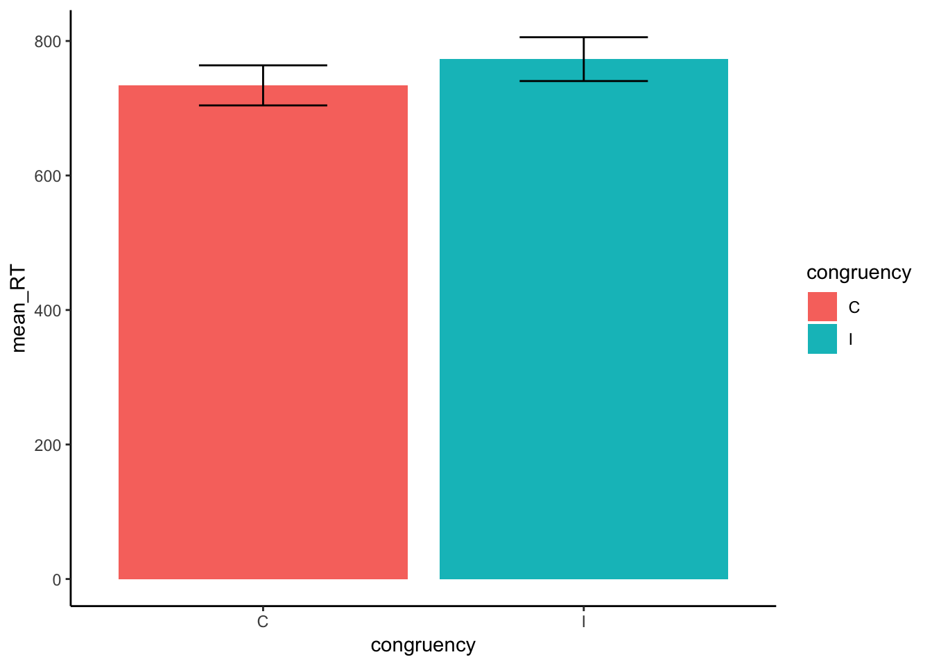
- Compute the flanker effect for each subject, taking the difference between their mean incongruent and congruent RT. Then plot the mean flanker effect, along with the SEM of the mean flanker effect
**tip:** Not all problems have an easy solution in dplyr, this is one them. You may have an easier time using logical indexing of the dataframe to solve this part.
Sub_flanker <- as.numeric(check[check$congruency=="I",]$mean_RT - check[check$congruency=="C",]$mean_RT)

Sub_means <- mean(Sub_flanker)
Sub_SEM <- sd(Sub_flanker)/sqrt(length(Sub_flanker))

Sub_flank<- data.frame(DV = "flanker effect", Sub_means, Sub_SEM)

ggplot(Sub_flank, aes(x = DV, y = Sub_means))+
  geom_bar(stat = "identity")+
  theme_classic(base_size = 14)+
  geom_errorbar(aes(ymin = Sub_means - Sub_SEM,
                    ymax = Sub_means + Sub_SEM),
                position = position_dodge(width = 1.2),
                width = .4, color = "green")+
  ylab("Mean Flanker Effect")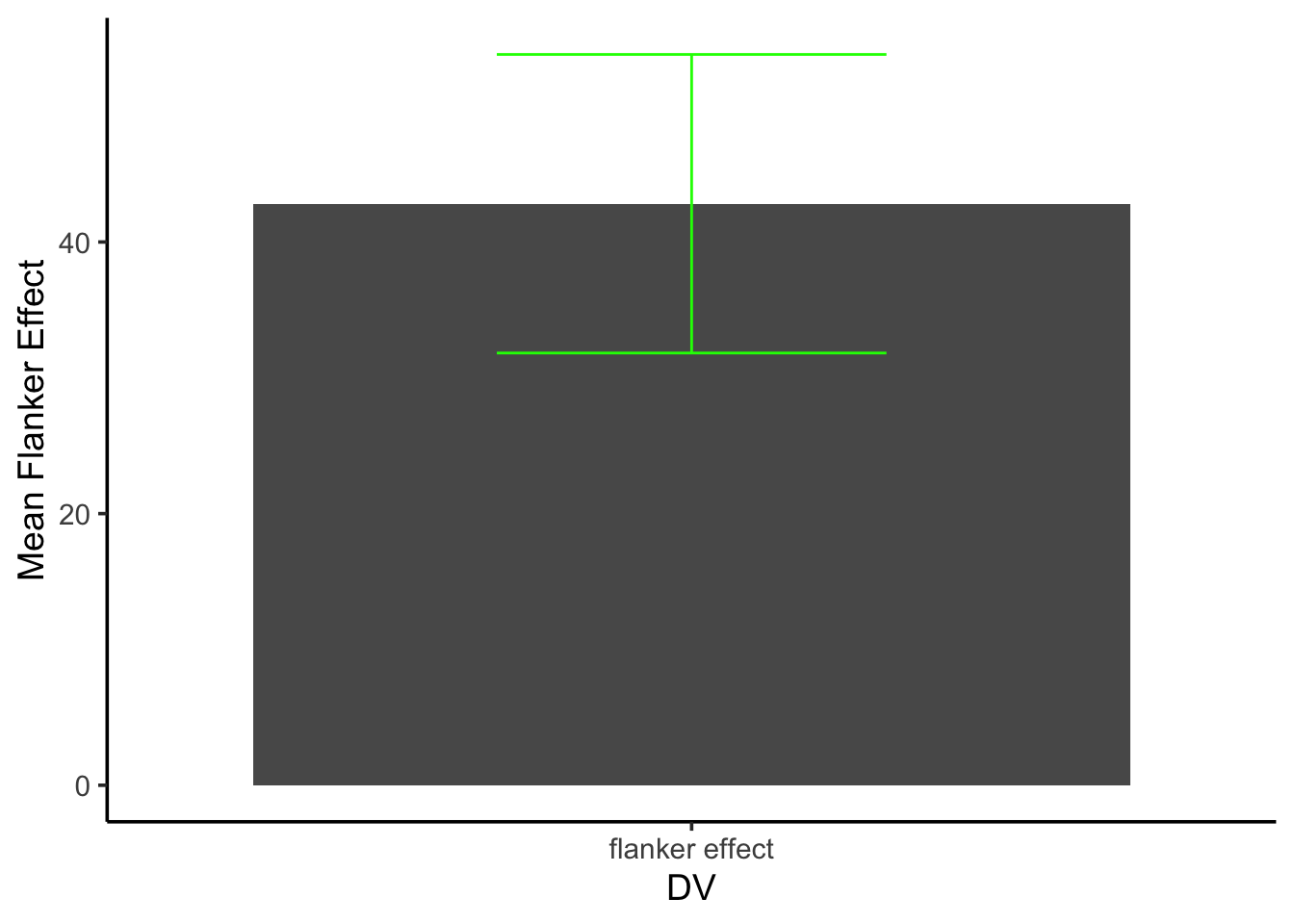
Exploratory analysis
Multiple questions may often be asked of data, especially questions that may not have been of original interest to the researchers.
In flanker experiments, like this one, it is well known that the flanker effect is modulated by the nature of the previous trial. Specifically, the flanker effect on trial n (the current trial), is larger when the previous trial (trial n-1) involved a congruent item, compared to an incongruent item.
Transform the data to conduct a sequence analysis. The dataframe should already include a factor (column) for the congruency level of trial n. Make another column that codes for the congruency level of trial n-1 (the previous trial). This creates a 2x2 design with trial n congruency x trial n-1 congruency.
First get teh subject means for each condition, then create a table and plot for teh overall means and SEMs in each condition. This should include:
- trial n congruent : trial n-1 congruent
- trial n incongruent : trial n-1 congruent
- trial n congruent : trial n-1 incongruent
- trial n incongruent : trial n-1 incongruent
**tip:** be careful, note that the first trial in each experiment can not be included, because it had no preceding trial